Adaptive Antennas and Receivers

Citation preview

DK6045_half-series-title

9/15/05

2:55 PM

Page i

Adaptive Antennas and Receivers

Edited By

Melvin M. Weiner The MITRE Corporation (Retired) Bedford, Massachusetts, U.S.A.

Boca Raton London New York

A CRC title, part of the Taylor & Francis imprint, a member of the Taylor & Francis Group, the academic division of T&F Informa plc.

© 2006 by Taylor & Francis Group, LLC

DK6045_Discl.fm Page 1 Monday, June 20, 2005 10:07 AM

Published in 2006 by CRC Press Taylor & Francis Group 6000 Broken Sound Parkway NW, Suite 300 Boca Raton, FL 33487-2742 © 2006 by Taylor & Francis Group, LLC CRC Press is an imprint of Taylor & Francis Group No claim to original U.S. Government works Printed in the United States of America on acid-free paper 10 9 8 7 6 5 4 3 2 1 International Standard Book Number-10: 0-8493-3764-X (Hardcover) International Standard Book Number-13: 978-0-8493-3764-2 (Hardcover) Library of Congress Card Number 2005043746 This book contains information obtained from authentic and highly regarded sources. Reprinted material is quoted with permission, and sources are indicated. A wide variety of references are listed. Reasonable efforts have been made to publish reliable data and information, but the author and the publisher cannot assume responsibility for the validity of all materials or for the consequences of their use. No part of this book may be reprinted, reproduced, transmitted, or utilized in any form by any electronic, mechanical, or other means, now known or hereafter invented, including photocopying, microfilming, and recording, or in any information storage or retrieval system, without written permission from the publishers. For permission to photocopy or use material electronically from this work, please access www.copyright.com (http://www.copyright.com/) or contact the Copyright Clearance Center, Inc. (CCC) 222 Rosewood Drive, Danvers, MA 01923, 978-750-8400. CCC is a not-for-profit organization that provides licenses and registration for a variety of users. For organizations that have been granted a photocopy license by the CCC, a separate system of payment has been arranged. Trademark Notice: Product or corporate names may be trademarks or registered trademarks, and are used only for identification and explanation without intent to infringe.

Library of Congress Cataloging-in-Publication Data Adaptive antennas and receivers / edited by Melvin M. Weiner. p. cm. -- (Electrical engineering and electronics ; 126) Includes bibliographical references and index. ISBN 0-8493-3764-X (alk. paper) 1. Adaptive antennas. I. Weiner, Melvin M. II. Series. TK7871.67.A33A32 2005 621.382'4--dc22

2005043746

Visit the Taylor & Francis Web site at http://www.taylorandfrancis.com Taylor & Francis Group is the Academic Division of T&F Informa plc.

© 2006 by Taylor & Francis Group, LLC

and the CRC Press Web site at http://www.crcpress.com

In memory of our parents, Kate and William Melvin and Donald Weiner

In memory of my wife, Clara Ronald Fante

© 2006 by Taylor & Francis Group, LLC

Preface The primary intent of this book is to provide an introduction to state-of-the art research on the modeling, testing, and application of adaptive antennas and receivers. As such, it provides a baseline for engineers, scientists, practitioners, and students in surveillance, communication, navigation, government service, artificial intelligence, computer tomography, neuroscience, and security intrusion industries. This book is based on work performed at Syracuse University and The MITRE Corporation with sponsorship primarily by the U. S. Air Force. At issue is the detection of target signals in a competing electromagnetic environment which is much larger than the signal after conventional signal processing and receiver filtering. The competing electromagnetic environment is external system noise (herein designated as “noise”) such as clutter residue, interference, atmospheric noise, man-made noise, jammers, external thermal noise (optical systems), in vivo surrounding tissue (biological systems), and surrounding material (intrusion detection systems). The environment is statistically characterized by a probability density function (PDF) which may be Gaussian, or more significantly, nonGaussian. For applications with an objective of target detection, the signal is assumed to be from a moving target within the surveillance volume and with a velocity greater than the minimum discernable velocity. In radars, which look down at the ground to detect targets, the clutter echo power can be 60 to 80 dB larger than the target echo power before signal processing. The target is detected by measuring the difference in returns from one pulse to the next. This method is based on the underlying assumption that the clutter echo power and the radar system are stable between pulses whereas the target signal is not. The degree of stability influences the subclutter visibility (SCV), i.e., the ratio by which the target echo power may be weaker than the coincident clutter echo power and still be detected with specified detection and false-alarm probabilities. The receiving systems of interest comprise an antenna array, digital receiver, signal processor, and threshold detector.1 The electromagnetic environment is assumed to be characterized by a “noise” voltage with a PDF that is temporally Gaussian but not necessarily spatially Gaussian. Conventional signal detection, for a specified false alarm rate or bit error rate, is achieved by measuring the magnitude-squared output of a linear Gaussian receiver compared to a single threshold determined by the variance of the noise voltage averaged over all the cells of the total surveillance volume. v © 2006 by Taylor & Francis Group, LLC

vi

Preface

A linear Gaussian receiver is defined as a receiver matched to the frequency spectrum of the signal and assumes a temporally Gaussian PDF “noise” voltage. In conventional signal detection, the probability of signal detection within any cell of the surveillance volume is small if the signal power is small compared to the average noise variance of the total surveillance volume. This book considers the more general case where the “noise” environment may be spatially nonGaussian. The book is divided into three parts where each part presents a different but sequentially complementary approach for increasing the probability of signal detection within at least some of the cells of the surveillance volume for a nonGaussian or Gaussian “noise” environment. These approaches are: Approach A. Homogeneous Partitioning of the Surveillance Volume; Approach B. Adaptive Antennas; and Approach C. Adaptive Receivers. Approach A. Homogeneous Partitioning of the Surveillance Volume. This approach partitions the surveillance volume into homogeneous, contiguous subdivisions. A homogeneous subdivision is one that can be subdivided into arbitrary subgroups, each of at least 100 contiguous cells, such that all the subgroups contain stochastic spatio-temporal “noise” sharing the same PDF. At least 100 cells/subgroup are necessary for sufficient confidence levels (see Section 4.3). The constant false-alarm rate (CFAR) method reduces to Approach A if the CFAR “reference” cells are within the same homogeneous subdivision as the target cell. When the noise environment is not known a priori, then it is necessary to sample the environment, classify and index the homogeneous subdivisions, and exclude those samples that are not homogeneous within a subdivision. If this sampling is not done in a statistically correct manner, then Approach A can yield disappointing results because the estimated PDF is not the actual PDF. Part I Homogeneous Partitioning of the Surveillance Volume addresses this issue. Approach B. Adaptive Antennas. This approach, also known as space-time adaptive processing, seeks to minimize the competing electromagnetic environment by placing nulls in its principal angle-of-arrival and Doppler frequency (space-time) domains of the surveillance volume. This approach utilizes k ¼ NM samples of the signals from N subarrays of the antenna over a coherent processing interval containing M pulses to (1) estimate, in the space-time domain, an NM £ NM “noise” covariance matrix of the subarray signals, (2) solve the matrix for up to N unknown “noise” angles of arrival and M unknown “noise” Doppler frequencies, and (3) determine appropriate weighting functions for each subarray that will place nulls in the estimated angle-of-arrival and Doppler frequency domains of the “noise”. Approach B is a form of filtering in those domains. Consequently, the receiver detector threshold can be reduced because the average “noise” voltage variance of the surveillance volume is reduced. The locations and depths of the nulls are determined by the relative locations and strengths of the “noise” sources in the space-time domain and by differences in the actual and estimated “noise” covariance matrices. The results are influenced by the finite number k of © 2006 by Taylor & Francis Group, LLC

Preface

vii

stochastic data samples and the computational efficiency in space-time processing the samples. Part II Adaptive Antennas addresses these issues and presents physical models of several applications. Approach C. Adaptive Receivers. For each homogeneous subdivision of the surveillance volume, this approach generally utilizes a nonlinear, nonGaussian receiver whose detection algorithm is matched to the sampled “noise” voltage spatial PDF of that subdivision. When the nonGaussian “noise” waveform is spikier than Gaussian noise, the nonlinear receiver is more effective than a linear receiver in reducing the detecton threshold for a given false alarm rate provided that the estimated spatial PDF is an accurate representation of the actual PDF. If the estimated spatial PDF is Gaussian, then the nonlinear receiver reduces to a linear Gaussian receiver. At issue are (1) how to model, simulate, and identify the random processes associated with the correlated “noise” data samples and (2) how to determine the nonlinear receiver and its threshold that are best matched to those data samples. Part III Adaptive Receivers addresses and illustrates these issues with some applications. Approach C should not be implemented until Approaches A and B have been implemented. For a prespecified false alarm probability, Approach A or B alone have a better probability of target detection than in their absence. The combination of Approaches A and B has a better probability of target detection than Approach A or B alone. The combination of Approaches A, B, and C has a still better probability of target detection. For this reason, this book often refers to the combination of Approaches A, B, and C as the weak signal problem, (i.e., small signal-to-noise ratio case); the combination of Approaches A and B or Approach A or B alone as the intermediate signal problem, (i.e., intermediate signal-to-noise ratio case); and the absence of all three approaches as the strong signal problem, (i.e., large signal-to-noise ratio case). Approaches A and C are usually more difficult to implement than Approach B alone because “noise” spatial PDF is more difficult to measure than “noise” variance. However, for the weak signal problem, Approaches A and C can be worth the effort as is shown in Part III. All of these approaches have benefited from orders-of-magnitude increases in the speeds of beam scanning and data processing made possible by recent technological advances in integrated circuits and digital computers. However, equally important, are the recent advances in methodology which are reported in this book. Adaptive antennas originated in the 1950s with classified work by S. Applebaum followed later by P. W. Howells, both of whom published their work about 40 years ago.2,3 Practical techniques for space-time processing of the sampled data originated with B. Widrow and colleagues approximately a year later.4 A nonlinear nonGaussian receiver for weak signal detection, in the presence of “noise” whose PDF is not necessarily Gaussian, originated with D. Middleton approximately 45 years ago.5 The receiver is designated a “locally optimum detector” (LOD) because, in a Taylor series expansion of the numerator of the likelihood ratio (LR) about a unity operating point, only the second term © 2006 by Taylor & Francis Group, LLC

viii

Preface

(a linear test statistic) is retained and the first term (a constant) is combined as part of the threshold. Thus, for small signal-to-disturbance ratio, a sensitive yet computationally simpler test statistic is obtained, resulting in either a nonlinear receiver for non-Gaussian disturbances or a linear matched filter for Gaussian disturbances with deterministic signals. Unlike an adaptive receiver, Middleton’s LOD utilized a fixed detection algorithm and threshold that were determined a priori to the detection process. The feasibility of an adaptive receiver was made possible less than 15 years ago when Aydin Ozturk (Professor, Dept. of Mathematics, Syracuse University) developed an algorithm for identifying and estimating univariate and multivariate distributions based on sample-order statistics.6,7 At that time, my brother, Donald D. Weiner (Professor, Dept. of Electrical and Computer Engineering, Syracuse University), in collaboration with his doctoral student Muralidhar Rangaswamy and A. Ozturk, conceived the idea of an adaptable receiver which (1) sampled in real time the “noise” environment, (2) utilized the Ozturk algorithm to estimate the “noise” PDF, and (3) utilized the Middleton LOD by matching its detection algorithm and threshold to the estimated “noise” PDF.8,9 By 1993, with additional collaboration from Prakash Chakravarthi, Mohamed-Adel Slamani (doctoral students of D. D. Weiner), Hong Wang (Professor, Dept. of Electrical and Computer Engineering, Syracuse University) and Lujing Cai (doctoral student of H. Wang), the core ideas for much of the material in this book had been developed.10,11 With the exception of Chapters 9 and 10, all of the materials in this book are based on later refinements, elaborations, and applications by D. D. Weiner, his students (Thomas J. Barnard, P. Chakravarthi, Braham Himed, Andrew D. Keckler, James H. Michels, M. Rangaswamy, Rajiv R. Shah, M. A. Slamani, Dennis L. Stadelman), his colleagues at Syracuse University (A. Ozturk, H. Wang), students of H. Wang (L. Cai, Michael C. Wicks), his colleagues at Rome Laboratory (Christopher T. Capraro, Gerard T. Capraro, David Ferris, William J. Baldygo, Vincent Vannicola), his son (William W. Weiner), and Fyzodeen Khan (colleague of T. J. Barnard). Chapter 9 is contributed by George Ploussios (consultant, Cambridge, MA). Chapter 10 consists of reprints of all the refereed journal papers on adaptive antennas individually authored by Ronald L. Fante (Fellow, The MITRE Corporation) or co-authored with colleagues Edward C. Barile, Richard M. Davis, Thomas P. Guella, Jose A. Torres, and John J. Vaccaro. My interest in the core ideas of this book originated in 1993 from two invited talks at the MITRE Sensor Center.12,13 The two talks utilized novel mathematical tools (such as the Ozturk algorithm and spherically invariant random vectors) for more effective implementation of homogeneous partitioning, adaptive antennas, and adaptive receivers. Since that time, the utilization of these tools for those purposes has been reported in the journal literature but not in a book. In July 2003, Marcel Dekker Inc. asked me to recommend a prospective author for a book on smart antennas. Smart antennas are nothing more than adaptive antennas (with or without the signal processing associated with adaptive © 2006 by Taylor & Francis Group, LLC

Preface

ix

antennas) which are specifically tailored for the wireless mobile communication industry. Since there were already several books on smart antennas, the publisher agreed instead to accept a proposal from me for the present book. All of the material for this book is in the public domain. Chapters 1, 7, 9, and 11 were written specifically for this book. The material is from the following sources: Chap. 1 2

3.1 3.2 4

5.1 5.2

6.1

6.2

6.3

Source Contributed by Weiner, M.M. Slamani, M.A., A New Approach to Radar Detection Based on the Partitioning and Statistical Characterization of the Surveillance Volume, University of Massachusetts at Amherst, Final Technical Report, Rome Laboratory, Air Force Material Command, RL-TR-95164, Vol. 5, Sept. 1995. Rangaswamy, M., Michels, J.H., and Himed, B., Statistical analysis of the nonhomogeneity detector for STAP applications, Digital Signal Processing Journal, Vol. 14, No. 1, Jan. 2004. Rangaswamy, M., Statistical analysis of the nonhomogeneity detector for nongaussian interference backgrounds, IEEE Trans. Signal Processing, Vol. 15, Jan./Feb. 2005. Shah, R.R., A New Technique for Distribution Approximation of Random Data, University of Massachusetts at Amherst, Final Technical Report, Rome Laboratory, Air Force Material Command, RL-TR-95-164, Vol. 2, Sept. 1995. Ozturk, A., A New Method for Distribution Identification, J. American Statistical Association, submitted but not accepted for publication, 1990 (revised 2004). Contributed by A. Ozturk. Ozturk, A., A general algorithm for univariate and multivariate goodness-of-fit tests based on graphical representation, Commun. in Statistics, Part A—Theory and Methods, Vol. 20, No. 10, pp. 3111– 3131, 1991. Weiner, W.W., The Ozturk Algorithm: A New Technique for Analyzing Random Data with Applications to the Field of Neuroscience, Math Exam Requirements for Ph.D. in Bioengineering and Neuroscience, Syracuse University, May 9, 1996. Slamani, M.A. and Weiner, D.D., Use of image processing to partition a radar surveillance volume into background noise and clutter patches, Proc. 1993 Conference on Information Sciences and Systems, Johns Hopkins Univ., Baltimore, Md., March 24 –26, 1993. Slamani, M.A. and Weiner, D.D., Probabilistic insight into the application of image processing to the mapping of clutter and noise regions in a radar surveillance volume, Proc. 36th Midwest Symposium of Circuits and Systems, Detroit, Mi., Aug. 10– 18, 1993.

© 2006 by Taylor & Francis Group, LLC

x

Preface

6.4 6.5

6.6

6.7

6.8

7 8

9 10.1 10.2 10.3 10.4 10.5 10.6 10.7

Slamani, M.A., Ferris, D., and Vannicola, V., A new approach to the analysis of IR images, Proc. 37th Midwest Symposium in Circuits and Systems, Lafayette, LA, Aug. 3– 5, 1994. Slamani, M.A., Weiner, D.D., and Vannicola, V., ASCAPE: An automated approach to the statistical characterization and partitioning of a surveillance volume, Proc. 6th International Conference on Signal Processing Applications and Technology, Boston, MA, Oct. 24–26, 1995. Keckler, A.D., Stadelman, D.L., Weiner, D.D., and Slamani, M.A., Statistical Characterization of Nonhomogeneous and Nonstationary Backgrounds, Aerosense 1997 Conference on Targets and Backgrounds: Characterization and Representation III, Orlando FL, April 21–24, 1997, SPIE Proceedings, Vol. 3062, pp. 31–40, 1997. Capraro, C.T., Capraro, G.T., Weiner, D.D., and Wicks, M.C., Knowledge-based map space-time adaptive processing, Proc. 2001 International Conference on Imaging Science, Systems, and Technology, Las Vegas, Nev., Vol. 2, pp. 533–538, June 2001. Capraro, C.T., Capraro, G.T., Weiner, D.D., Wicks, M.C., and Baldygo, W.J., Improved space-time adaptive processing using knowledge-aided secondary data selection, Proc. 2004 IEEE Radar Conference, Philadelphia, PA, April 26–29, 2004. Contributed by Weiner M.M. Cai, L. and Wang, H., Adaptive Implementation of Optimum SpaceTime Processing, Chapter 2, Kaman Sciences Corp., Final Technical Report, Rome Laboratory, Air Force Material Command, RL-TR-9379, May 1993. Contributed by Ploussios, G. Fante, R.L., Cancellation of specular and diffuse jammer multipath using a hybrid adaptive array, IEEE Trans. Aerospace and Electronic Systems, Vol. 27, No. 5, pp. 823–837, Sept. 1991. Barile, E., Fante, R.L., and Torres, J., Some Limitations on the effectiveness of airborne adaptive radar, IEEE Trans. Aerospace and Electronic Systems, Vol. 28, No. 4, pp. 1015–1032, Oct. 1992. Fante, R.L., Barile, E., and Guilla, T., Clutter covariance smoothing by subaperture averaging, IEEE Trans. Aerospace and Electronic Systems, Vol. 30, No. 3, pp. 941–945, July 1994. Fante, R.L. and Torres, J., Cancellation of diffuse jammer multipath by an airborne adaptive radar, IEEE Trans. Aerospace and Electronic Systems, Vol. 31, No. 2, pp. 805–820, April 1995. Fante, R.L., Davis, R.M., and Guella, T.P., Wideband cancellation of multiple mainbeam jammers, IEEE Trans. Antennas and Propagation, Vol. 44, No. 10, pp. 1402–1413, Oct. 1996. Fante, R.L., Adaptive space-time radar, J. Franklin Inst., Vol. 335B, pp. 1–11, Jan. 1998. Fante, R.L., Synthesis of adaptive monopole patterns, IEEE Trans. Antennas and Propagation, Vol. 47, No. 5, pp. 773–774, May 1999.

© 2006 by Taylor & Francis Group, LLC

Preface

10.8 10.9 10.10 10.11 11 12

13

14 15.1 15.2 15.3

15.4

15.5 15.6

xi

Fante, R.L., Ground and airborne target detection with bistatic adaptive space-based radar, IEEE AES Systems Magazine, pp. 39–44, Oct. 1999. Fante, R.L., Adaptive nulling of SAR sidelobe discretes, IEEE Trans. Aerospace and Electronic systems, Vol. 35, No. 4, pp. 1212–1218, Oct. 1999. Fante, R.L. and Vaccaro, J.J., Wideband cancellation of interference in a GPS receive array, IEEE Trans. Aerospace and Electronic Systems, Vol. 36, No. 2, pp. 549–564, April 2000. Davis, R.M. and Fante, R.L., A maximum likelihood beamspace processor for improved search and trace, IEEE Trans. Antennas and Propagation, Vol. 49, No. 7, pp. 1043–1053, July 2001. Contributed by Weiner, M.M. Rangaswamy, M., Spherically Invariant Random Processes and Radar Clutter Modeling, Simulation, and Distribution Identification, Final Technical Report, Rome Laboratory, Air Force Materiel Command, RL-TR-95-164, Vol. 3, Sept. 1995. Chakravarthi, P., The Problem of Weak Signal Detection, University of Massachusetts at Amhest, Final Technical Report, Rome Laboratory, Air Force Materiel Command, RL-TR-95-164, Vol. 4, Sept. 1995. Barnard, T.J., A Generalization of Spherically Invariant Random Vectors with an Application to Reverberation Reduction in a Correlation Radar, Ph.D. Thesis, Syracuse University, April 1994. Barnard, T.J. and Khan, F., Statistical normalization of spherically invariant nonGaussian clutter, IEEE J. Oceanic Eng., 29(2):303–309, April 2004. Keckler, A.D., Stadelman, D.L., and Weiner, D.D., NonGaussian clutter modeling and application to radar detection, Proc. 1997 IEEE National Radar Conference, Syracuse, N. Y., May 13–15, 1997. Stadelman, D.L., Keckler, A.D., and Weiner, D.D., Adaptive Ozturkbased receivers for small signal detection in impulsive nonGaussian clutter, 1999 Conference on Signal and Data Processing of Small Targets, SPIE Proc., Vol. 3809, Denver CO, July 20–22, 1999. Stadelman, D.L., Weiner, D.D., and Keckler, A.D., Efficient determination of thresholds via importance sampling for monte carlo evaluation of radar performance in nonGaussian clutter, Proc. 2002 IEEE Radar Conference, Long Beach, CA, April 22–25, 2002. Keckler, A.D. and Weiner, D.D., Generation of rejection method bounds for spherically invariant random vectors, Proc. 2002 IEEE Radar Conference, Long Beach, CA, April 22–25, 2002. Stadelman, D. and Weiner, D.D., Optimal NonGaussian Processing in Spherically Invariant Interference, Syracuse University, Final Technical Report, Air Force Research Laboratory, AERL-SN-RS-TR-1998–26, March 1998.

© 2006 by Taylor & Francis Group, LLC

xii

15.7

Preface

Rangaswamy, M., Michels, J.H., and Weiner, D.D., Multichannel detection for correlated nonGaussian random processes based on innovations, IEEE Trans. Signal Processing, Vol. 43, No. 8, pp. 1915–1995, August 1995. Melvin M. Weiner Editor

© 2006 by Taylor & Francis Group, LLC

Biography Melvin M. Weiner received S.B. and S.M. degrees in electrical engineering from Massachusetts Institute of Technology in 1956 (Cooperative Honors Program). From 1953 to 1956 he was a co-op student at Philco Corp., Philadelphia, working on cathode-ray tubes. From 1956 until the present, he has been engaged in the Boston area in the fields of electromagnetics, physical electronics, optics, lasers, communications, and radar systems. He served as project engineer at Chu Associates (1956 to 1959) on ferrite phase shifters and electronic scanning antennas; senior engineer at EG&G, Inc. (1963 to 1966) on optical detection of high-altitude nuclear explosions; senior staff engineer at Honeywell Radiation Center (1966 to 1967) on infrared surveillance systems and fluxgate magnetometers; staff engineer at AS&E, Inc. (1967 to 1968) on x-ray telescopes, gammaray spark chambers, and Cockcroft-Walton voltage multipliers; consulting inventor (1959 to 1971) of the traveling-wave cathode ray tube, nonimaging solar concentrator, first continuous-wave solid-state laser, and first photonic crystal and holey fiber; principal research engineer at AVCO Everett Research Laboratory (1971 to 1978) on optical design and diagnostics of high power CO2 lasers including co-invention of the off-axis unstable resonator; member of the technical staff at The MITRE Corp. (1978 to 1994) on bistatic radar phenomenology, airborne anti-jam VHF radios, and ground-based over-thehorizon HF radar systems; and author (1994 to present) of two of his three books on electomagnetics, with three additional books in preparation. He is the author of 36 refereed papers, one book chapter, three books (Monopole Elements on Circular Ground Planes, Norwood, MA: Artech House, 1987; Monopole Antennas, New York: Marcel Dekker, 2003; Adaptive Antennas and Receivers, New York: Marcel Dekker, 2005) and holder of five U. S. patents. Mr. Weiner is a member of the Institute of Electrical and Electronics Engineers, Optical Society of America; Sigma Xi, and Eta Kappa Nu of which he was a national director (1969 to 1971) and founder-chairman of the Motor Vehicle Safety Group (1969 to 1973) contributing to the establishment of the current National Highway Traffic Safety Administration.

xiii © 2006 by Taylor & Francis Group, LLC

Acknowledgments The 29 contributing authors to this book are from four groups of sources. Chapters 1, 7, and 11 were contributed by the Editor. All the other chapters except Chapter 9 and Chapter 10 were solicited from the Editor’s brother D. D. Weiner and D.D. Weiner’s doctoral students, colleagues at Syracuse University and U. S. Air Force Rome Laboratory, and son. Chapter 9 was solicited from G. Ploussios, the Editor’s former MIT classmate and colleague at Chu Associates and The MITRE Corporation. Chapter 10 was solicited from R. L. Fante, the Editor’s former colleague at The MITRE Corporation. Chapter 2 was supported by U. S. Air Force Rome Laboratory under Contract UM915025/28140. Constructive suggestions and contributions were received from D. D. Weiner, P. Varshney, H. Wang, C. Isik of Syracuse University; L. Slaski, V. Vannicola of Rome Laboratory; V. Lesser of University of Massachusetts; and H. Nawab of Boston University (IPUS Program). Chapter 3 was supported by the U. S. Air Force Office of Scientific Research under Projects 2304E8, 2304IN, and by in-house research efforts at the U. S. Air Force Research Laboratory. Chapter 4 was supported by the U. S. Air Force Rome Laboratory under Contract F30602-91-C-0038. Constructive suggestions and contributions were received from D. D. Weiner, L. Slaski, P. Chakravarthi, M. Rangaswamy, and M. Slamani. Support from the Computer Applications and Software Engineering (CASE) Center of Syracuse University is also gratefully acknowledged. Chapter 5 was supported in part by the National Science Foundation under Grant No. G88135. Support from the Computer Applications and Software Engineering (CASE) Center of Syracuse University is also gratefully acknowledged. Chapter 6: Section 6.1 received constructive suggestions from R. Smith, D. D. Weiner, S. Chamberlain, E. Relkin, C. Passaglia, M. Slamani, and M. Schecter of Syracuse University. Section 6.2 and Section 6.3 were supported by the U. S. Air Force Rome Laboratory under Contract F30602-91-C-0038. Section 6.4 was supported by the U. S. Air Force Office of Scientific Research under Rome Laboratory Contract AF30602-94-C-0203. Section 6.5 was supported by the U. S. Air Force Rome Laboratory and received constructive suggestions and contributions from J. Michels, M. Rangaswamy, H. Hottelet, C. Zamara, B. Testa, and D. Hui. Section 6.6 was supported in part by the U. S. AFRL Sensors Directorate under Contract F30602-97-C-0065 and received constructive suggestions from G. Genello. xv © 2006 by Taylor & Francis Group, LLC

xvi

Acknowledgments

Chapter 8 was supported by the U. S. Air Force Rome Laboratory under Contract F30602-89-C-0082. Chapter 10: Section 10.1 and Section 10.2 were supported by the U. S. Air Force Electronic Systems Division under Contract F19628-89-C-0001 and received constructive suggestions and contributions from K. Gude, R. Games (Section 10.1); R. Dipietro, B. N. Suresh Babu, T. Guella, D. Lamensdorf, S. Townes (Section 10.2). Sections 10.3 to 10.10 received constructive suggestions and contributions from R. DiPietro, D. Lamensdorf, J. A. Torres (Section 10.3); R. Martin of Westinghouse, E. Barile, D. Lamensdorf, B. N. Suresh Babu, R. DiPietro, T. Guella, R. Williams (Section 10.4); T. Hopkinson, J. Torres, D. Moulin, R. DiPietro, J. Williams, R. Rama Rao (Section 10.10). Chapter 12 was supported by the U. S. Air Force Rome Laboratory under Contracts SCEE-DACS-P35498-2, UM 91S025/2810, and F30602-91C-0038. Constructive suggestions and contributions were received from D. D. Weiner, R. Srinivasan, A. Ozturk, L. Slaski, R. Brown, M. Wicks, J. H. Michels, P. Chakravarthi, T. Sarkar, and H. Schwarzlander. Support from the Academic Computing Services of Syracuse University is also gratefully acknowledged. Chapter 13 was supported by the U. S. Air Force Rome Laboratory under Contracts SCEE-DACS-P35498-2, UM 91S025/28140, and F30602-91-C-0038. Constructive suggestions and contributions were received from D. D. Weiner, R. Srinivasan, A. Ozturk, M. Rangaswamy, and M. Slamani of Syracuse University; and M. Wicks, R. Brown, L. Slaski, and Michels of Rome Laboratory. Chapter 14 received constructive suggestions and contributions from A. Ozturk, M. Rangaswamy, D. D. Weiner, and the Martin Marietta Corporation. Chapter 15: Section 15.2 was supported by the U. S. Air Force Rome Laboratory through the Office of Scientific Research Summer Graduate Student Research Program and received constructive suggestions and contributions from J. Michels, M. Rangaswamy, H. Hottelet, C. Zamora, B. Testa, and D. Hui. Section 15.5 was supported in part by the U. S. Air Force Rome Laboratory through the Office of Scientific Research Summer Graduate Student Research Program and received constructive suggestions and contributions from J. Michels, M. Rangaswamy, and D. Stadelman. Section 15.6 was supported by the Advanced Research Projects Agency of the U. S. Dept. of Defense under Contract F3060294-C-0287 and received constructive suggestions and contributions from H. Hottelet, D. Hui, A. Keckler, E. J. Dudewicz, and F. Sezgin. Section 15.7 was supported by the U. S. Air Force Office of Scientific Research under Project 2304E8 and the U. S. Air Force Rome Laboratory in-house effort under Project 4506, and received constructive suggestions and contributions from R. Vienneau, T. Robbins, R. Srinivasan, and J. Lennon. Some of the material in this book has been published in refereed journals, conference proceedings, or other public domains protected by copyright. Receipt of waiver of copyright is gratefully acknowledged as follows: © 2006 by Taylor & Francis Group, LLC

Acknowledgments

xvii

CHAPTER 3 Rangaswamy, M., Michels, J.H., and Himed, B., Statistical analysis of the nonhomogeneity detector for STAP applications, Digital Signal Processing Journal, Vol. 14, No. 3, May 2004, pp. 253 –267. Rangaswamy, M., Statistical analysis of the nonhomogeneity detector for nonGaussian interference backgrounds, IEEE Trans. Signal Processing, Vol. 53, No. 6, June 2005, pp.2101 –2111.

CHAPTER 5 Ozturk, A., A general algorithm for univariate and multivariate goodness-of-fit tests based on graphical representation, Commun. in Statistics, Part A – Theory and Methods, Vol. 20, No. 10, 1991, pp. 3111– 3131.

CHAPTER 6 Weiner, W.W., The Ozturk Algorithm: A New Technique for Analyzing Random Data with Applications to the Field of Neuroscience, Math Exam Requirements for PhD in Bioengineering and Neuroscience, Syracuse University, May 9, 1996. Slamani, M.A. and Weiner, D.D., Use of image processing to partition a radar surveillance volume into background noise and clutter patches, Proc. 1993 Conference on Information Sciences and Systems, Johns Hopkins University, Baltimore, MD, March 24 –26, 1993. Slamani, M.A. and Weiner, D.D., Probabilistic insight into the application of image processing to the mapping of clutter and noise regions in a radar surveillance volume, Proc. 36th Midwest Symposium of Circuits and Systems, Detroit, MI, Aug. 10 – 18, 1993. Slamani, M.A., Ferris, D., and Vannicola, V. A new approach to the analysis of IR images, Proc. 37th Midwest Symposium in Circuits and Systems, Lafayette, LA, Aug. 3 –5, 1994. Slamani, M.A., Weiner, D.D., and Vannicola, V., ASCAPE: An automated approach to the statistical characterization and partitioning of a surveillance volume, Proc. 6th International Conference on Signal Processing Applications and Technology, Boston, MA, Oct. 24 –26, 1995. Keckler, A.D., Stadelman, D.L., Weiner, D.D., and Slamani, M.A., Statistical Characterization of Nonhomogeneous and Nonstationary Backgrounds, Aerosense 1997 Conference on Targets and Backgrounds: Characterization and Representation III, SPIE Proceedings, Vol. 3068, Orlando, FL, April 21 –24, 1997. Capraro, C.T., Capraro, G.T., Weiner, D.D., and Wicks, M.C., Knowledge-based map space-time adaptive processing, Proc. International Conference on Imaging Science, Systems, and Technology, Las Vegas, Nev., June 2001, Vol. 2, pp. 533 – 538. © 2006 by Taylor & Francis Group, LLC

xviii

Acknowledgments

Capraro, C.T., Capraro, G.T., Weiner, D.D., and Wicks, M.C., Improved spacetime adaptive processing using knowledge-aided secondary data selection, Proc. 2004 IEEE Radar Conference, Philadelphia, April 26– 29, 2004.

CHAPTER 10 Fante, R.L., Cancellation of specular and diffuse jammer multipath using a hybrid adaptive array, IEEE Trans. Aerospace and Electronic Systems, Vol. 27, No. 5, Sept. 1991, pp. 823– 837. Barile, E., Fante, R.L., and Torres, J. Some limitations on the effectiveness of airborne adaptive radar, IEEE Trans. Aerospace and Electronic Systems, Vol. 28, No. 4, Oct. 1992, pp. 1015– 1032. Fante, R.L., Barile, E., and Guilla, T., Clutter covariance smoothing by subaperture averaging, IEEE Trans. Aerospace and Electronic Systems, Vol. 30, No. 3, July 1994, pp. 941 – 945. Fante, R.L. and Torres, J., Cancellation of diffuse jammer multipath by an airborne adaptive radar, IEEE Trans. Aerospace and Electronic Systems, Vol. 31, No. 2, April 1995, pp. 805 –820. Fante, R.L., Davis, R.M., and Guella, T.P., Wideband cancellation of multiple mainbeam jammers, IEEE Trans. Antennas and Propagation, Vol. 44, No. 10, Oct. 1996, pp. 1402 –1413. Fante, R.L., Adaptive space-time radar, J. Franklin Inst., Vol. 335B, Jan. 1998, pp. 1 –11. Fante, R.L., Synthesis of adaptive monopole patterns, IEEE Trans. Antennas and Propagation, Vol. 47, No. 5, May 1999, pp. 773 – 774. Fante, R.L., Ground and airborne target detection with bistatic adaptive spacebased radar, IEEE AES Systems Magazine, Oct. 1999, pp. 39 – 44. Fante, R.L., Adaptive nulling of SAR sidelobe discretes, IEEE Trans. Aerospace and Electronic Systems, Vol. 35, No. 4, Oct. 1999, pp. 1212– 1218. Fante, R.L. and Vaccaro, J.J., Wideband cancellation of interference in a GPS receive array, IEEE Trans. Aerospace and Electronic Systems, Vol. 36, No. 2, April 2000, pp. 549 –564. Davis, R.M. and Fante, R.L., A maximum likelihood beamspace processor for improved search and trace, IEEE Trans. Antennas & Propagation, Vol. 49, No. 7, July 2001, pp. 1043 – 1053.

CHAPTER 15 Barnard, T.J. and Khan, F., Statistical normalization of spherically invariant nonGaussian clutter, IEEE J. Oceanic Eng., Vol. 29, No. 2, April 2004, pp. 303 –309. Keckler, A.D., Stadelman, D.L., and Weiner, D.D., NonGaussian clutter modeling and application to radar target detection, Proc. 1997 IEEE National Radar Conference, Syracuse, N Y., May 13 – 15, 1997. © 2006 by Taylor & Francis Group, LLC

Acknowledgments

xix

Stadelman, D.L., Keckler, A.D., and Weiner, D.D., Adaptive Ozturk-based receivers for small signal detection in impulsive nonGaussian clutter, 1999 Conference on signal and Data Processing of Small Targets, SPIE Proceedings, Vol. 3809, Denver, CO, July 20 –22, 1999. Stadelman, D.L., Weiner, D.D., and Keckler, A.D., Efficient determination of thresholds via importance sampling for monte carlo evaluation of radar performance in nonGaussian clutter, Proc. 2002 IEEE Radar Conference, Long Beach, CA, April 22 – 25, 2002. Keckler, A.D. and Weiner, D.D. Generation of rejection method bounds for spherically invariant random vectors, Proc. 2002 IEEE Radar Conference, Long Beach, CA, April 22 – 25, 2002. Rangaswamy, M., Michels, J.H., and Weiner, D.D., Multichannel detection for correlated nonGaussian random processes based on innovations, IEEE Trans. Signal Processing, Vol. 43, No. 8, August 1995, pp. 1915– 1995. The acquisition and production stages of this book were skillfully guided by B. J. Clark of Marcel Dekker and Nora Konopka, Theresa Delforn, and Gerry Jaffe of Taylor & Francis, respectively. Layout was magnificently managed by Carol Cooper of Alden Prepress Services UK.

© 2006 by Taylor & Francis Group, LLC

Contributors W. J. Baldygo U.S. Air Force Research Lab Rome, New York

D. Ferris U.S. Air Force Research Lab Rome, New York

E. C. Barile Raytheon Missile Defense Center Woburn, Massachusetts

T. P. Guella The MITRE Corp. Bedford, Massachusetts

T. J. Barnard Lockheed Martin Maritime Systems Syracuse, New York

B. Himed U.S. Air Force Research Lab Rome, New York

L. Cai Globespan Semiconductor, Inc. Redbank, New Jersey

A. D. Keckler Sensis Corp. DeWitt, New York

C. T. Capraro Capraro Technologies Utica, New York

F. Khan Naval Undersea Warfare Center Newport, Rhode Island

G. T. Capraro Capraro Technologies Utica, New York

J. H. Michels U.S. Air Force Research Lab Rome, New York

P. Chakravarthi Eka Systems Germantown, Maryland

A. Ozturk Ege University, Bornova, Izmir, Turkey

R. M. Davis The MITRE Corp. Bedford, Massachusetts

G. Ploussios Consultant Boston, Massachusetts

R. L. Fante The MITRE Corp. Bedford, Massachusetts

M. Rangaswamy U.S. Air Force Research Lab Hanscom AFB, Massachusetts xxi

© 2006 by Taylor & Francis Group, LLC

xxii

Contributors

R. R. Shah Juhu S., India

H. Wang Syracuse University Syracuse, New York

M. A. Slamani ITT Industries Alexandria, Virginia

D. D. Weiner Syracuse University (retired) Syracuse, New York

D. L. Stadelman Syracuse Research Corp. Syracuse, New York

M. M. Weiner The MITRE Corp. (retired) Bedford, Massachusetts

J. A. Torres The MITRE Corp. Bedford, Massachusetts

W. W. Weiner Rose-Hulman Institute of Technology Terra Haute, Indiana

J. J. Vaccaro The MITRE Corp. Bedford, Massachusetts V. Vannicola Research Associates for Defense Conversion Rome, New York

© 2006 by Taylor & Francis Group, LLC

M. C. Wicks U.S. Air Force Research Lab Rome, New York

Table of Contents Part I

Homogeneous Partitioning of the Surveillance Volume Chapter 1

Introduction .....................................................................................3

M. M. Weiner Chapter 2

A New Approach to Radar Detection Based on the Partitioning and Statistical Characterization of the Surveillance Volume ............................................................5

M. A. Slamani Chapter 3

Statistical Analysis of the Nonhomogeneity Detector (for Excluding Nonhomogeneous Samples from a Subdivision).................................................................................175

M. Rangaswamy, J. H. Michels, and B. Himed Chapter 4

A New Technique for Univariate Distribution Approximation of Random Data.................................................205

R. R. Shah Chapter 5

Probability Density Distribution Approximation and Goodness-of-Fit Tests of Random Data .....................................259

A. Ozturk Chapter 6

Applications.................................................................................295

W. J. Baldygo, C. T. Capraro, G. T. Capraro, D. Ferris, A. D. Keckler, M. A. Slamani, D. L. Stadelman, V. Vannicola, D. D. Weiner, W. W. Weiner, and M. C. Wicks

xxiii © 2006 by Taylor & Francis Group, LLC

xxiv

Table of Contents

Part II

Adaptive Antennas Chapter 7

Introduction .................................................................................419

M. M. Weiner Chapter 8

Adaptive Implementation of Optimum Space – Time Processing....................................................................................421

L. Cai and H. Wang Chapter 9

A Printed-Circuit Smart Antenna with Hemispherical Coverage for High Data-Rate Wireless Systems ......................439

G. Ploussios Chapter 10

Applications...............................................................................443

E. C. Barile, R. M. Davis, R. L. Fante, T. P. Guella, J. A. Torres, and J. J. Vaccaro

Part III

Adaptive Receivers Chapter 11

Introduction ...............................................................................603

M. M. Weiner Chapter 12

Spherically Invariant Random Processes for Radar Clutter Modeling, Simulation, and Distribution Identification..............................................................................605

M. Rangaswamy Chapter 13

Weak Signal Detection .............................................................707

P. Chakravarthi Chapter 14

A Generalization of Spherically Invariant Random Vectors (SIRVs) with an Application to Reverberation Reduction in a Correlation Sonar .............................................799

T. J. Barnard

© 2006 by Taylor & Francis Group, LLC

Table of Contents

Chapter 15

xxv

Applications...............................................................................913

T. J. Barnard, A. D. Keckler, F. Khan, J. H. Michels, M. Rangaswamy, D. L. Stadelman, and D. D. Weiner Appendices.....................................................................................................1039 Acronyms .......................................................................................................1117 References......................................................................................................1133 Computer Programs available at CRC Press Website.............................1169

© 2006 by Taylor & Francis Group, LLC

Part I Homogeneous Partitioning of the Surveillance Volume

© 2006 by Taylor & Francis Group, LLC

1

Introduction M. M. Weiner

Part I Homogeneous Partitioning of the Surveillance Volume discusses the implementation of the first of three sequentially complementary approaches for increasing the probability of target detection within at least some of the cells of the surveillance volume for a spatially nonGaussian or Gaussian “noise” environment that is temporally Gaussian. This approach, identified in the Preface as Approach A, partitions the surveillance volume into homogeneous contiguous subdivisions. A homogeneous subdivision is one that can be subdivided into arbitrary subgroups, each of at least 100 contiguous cells, such that all the subgroups contain stochastic spatio-temporal “noise” sharing the same probability density function (PDF). At least one hundred cells per subgroup are necessary for sufficient confidence levels (see Section 4.3). The constant falsealarm rate (CFAR) method reduces to Approach A if the CFAR “reference” cells are within the same homogeneous subdivision as the target cell. When the noise environment is not known a priori, then it is necessary to sample the environment, classify and index the homogeneous subdivisions, and exclude samples that are not homogeneous within a subdivision. If this sampling is not done in a statistically correct manner, then Approach A can yield disappointing results because the estimated PDF is not the actual PDF. Part I addresses this issue. Chapter 2 discusses the implementation of Approach A to the radar detection problem. In Section 2.1, the simplest but least versatile implementation is discussed for utilization when statistical knowledge of the environment is known a priori. Section 2.2 discusses a feedforward expert system for implementation when the statistical environment is not known a priori but must be estimated from data samples in real time. Section 2.3 introduces a feedback expert system Integrated Processing and Understanding of Signals (IPUS) that augments the feedforward system of Section 2.2 by assessing whether correct signal processing and understanding have taken place and then performs additional data sampling and signal processing if required. Section 2.4 discusses the application of a feedback expert system to radar signal processing. The issues associated with clutter-patch mapping (Section 2.5) and indexing (Section 2.6) with a feedforward expert system are implemented by IPUS for a feedback expert

3 © 2006 by Taylor & Francis Group, LLC

4

Adaptive Antennas and Receivers

system in Section 2.7. Conclusions and suggestions for future research are presented in Section 2.8. Chapter 3 analyzes the integrity of a nonhomogeneous detector (NHD) for excluding nonhomogeneous samples from a candidate subdivision. The cases of Gaussian and nonGaussian interference environments are discussed in Section 3.1 and Section 3.2, respectively. Given a finite number of correlated samples that are realizations of a stochastic process, as in Section 2.2 to Section 2.7 and Chapter 3, how does one determine the best-fit approximation to the PDF of those samples? Chapter 4 discusses a new technique, the Ozturk algorithm, for achieving this difficult task. After a review of the literature (Section 4.1), the Ozturk algorithm is summarized (Section 4.2), and then evaluated by simulation results (Section 4.3). Conclusions and suggestions for future work are given in Section 4.4. A more complete discussion of the Ozturk algorithm is given in Chapter 5 by its originator, Aydin Ozturk. Chapter 6 presents applications of homogeneous partitioning to neuroscience (Section 6.1), radar detection (Section 6.2, Section 6.3, Section 6.7, and Section 6.8), infra-red image processing (Section 6.4 and Section 6.5), and concealed weapon detection (Section 6.6). Section 6.2 and Section 6.3 summarize an image processing mapping procedure, previously discussed in Section 2.4 to Section 2.7, for distinguishing patches dominated by background noise from those dominated by clutter. Section 6.5 presents a formalized process Automatic Statistical Characterization and Partitioning of Environments (ASCAPE) for that purpose. Section 6.7 and Section 6.8 utilize a priori knowledge-based terrain maps to achieve homogeneous partitioning.

© 2006 by Taylor & Francis Group, LLC

2

A New Approach to Radar Detection Based on the Partitioning and Statistical Characterization of the Surveillance Volume M. A. Slamani

CONTENTS 2.0. Introduction.................................................................................................. 7 2.1. Radar Detection with a Priori Statistical Knowledge of the Environment ...................................................................................... 8 2.1.1. Introduction ....................................................................................... 8 2.1.2. SIRV ................................................................................................ 10 2.1.2.1. Definitions.......................................................................... 10 2.1.2.2. Properties of SIRVs ........................................................... 11 2.1.3. Locally Optimum Detector ............................................................. 12 2.2. Understanding of Signal and Detection Using a Feedforward Expert System ............................................................................................ 13 2.2.1. Introduction ..................................................................................... 13 2.2.2. Classification of the Test Cells ....................................................... 14 2.2.2.1. Mapping of the Space........................................................ 14 2.2.2.2. Indexing of the Cells ......................................................... 15 2.2.3. Target Detection .............................................................................. 16 2.3. Signal Understanding and Detection Using a Feedback Expert System ............................................................................................ 20 2.3.1. Introduction ..................................................................................... 20 2.3.2. IPUS Architecture ........................................................................... 20 2.3.2.1. Introduction........................................................................ 20

5 © 2006 by Taylor & Francis Group, LLC

6

Adaptive Antennas and Receivers

2.3.2.2. Discrepancy Detection....................................................... 24 2.3.2.3. Diagnosis and Reprocessing.............................................. 25 2.3.2.4. Interpretation Process ........................................................ 26 2.3.2.5. SOU and Resolving Control Structure.............................. 26 2.3.3. Application of IPUS to Radar Signal Understanding..................... 29 2.4. Proposed Radar Signal Processing System Using a Feedback Expert System ............................................................................................ 29 2.4.1. Data Collection and Preprocessing ................................................. 29 2.4.2. Mapping........................................................................................... 32 2.5. Mapping Procedure.................................................................................... 36 2.5.1. Introduction ..................................................................................... 36 2.5.2. Observations on BN and CL Cells.................................................. 37 2.5.2.1. Observations on BN Cells ................................................. 37 2.5.2.2. Observations on CL Cells ................................................. 38 2.5.3. Mapping Procedure ......................................................................... 39 2.5.3.1. Separation of CL Patches from Background Noise ............................................................. 39 2.5.3.2. Detection of CL Patch Edges and Edge Enhancement...................................................................... 44 2.5.3.3. Conclusion ......................................................................... 46 2.5.4. Examples of the Mapping Procedure.............................................. 47 2.5.4.1. Introduction........................................................................ 47 2.5.4.2. Examples............................................................................ 49 2.5.5. Convergence of the Mapping Procedure ........................................ 70 2.5.5.1. Introduction........................................................................ 70 2.5.5.2. Separation between BN and CL Patches .......................... 73 2.5.6. Extension of the Mapping Procedure to Range – Azimuth –Doppler Cells..................................................... 79 2.5.7. Conclusion ....................................................................................... 81 2.6. Indexing Procedure .................................................................................... 82 2.6.1. Introduction ..................................................................................... 82 2.6.2. Assessment Stage ............................................................................ 83 2.6.2.1. Identification of the BN and CL Patches .......................... 83 2.6.2.2. Computation of CL-to-Noise Ratios ................................. 85 2.6.2.3. Classification of CL Patches ............................................. 85 2.6.3. CL Subpatch Investigation Stage.................................................... 86 2.6.4. PDF Approximation of WSC CL Patches ...................................... 87 2.6.4.1. Test Cell Selection............................................................. 88 2.6.4.2. PDF Approximation........................................................... 89 2.6.4.3. PDF Approximation Metric............................................... 91 2.6.4.4. Outliers............................................................................... 93 2.6.4.5. PDF Approximation Strategy ............................................ 96 2.6.5. Examples ......................................................................................... 97 2.6.5.1. Example 1 .......................................................................... 97 2.6.5.2. Example 2 ........................................................................ 104 © 2006 by Taylor & Francis Group, LLC

A New Approach to Radar Detection

7

2.6.5.3. Example 3 ........................................................................ 106 2.6.6. Extension of the Indexing Procedure to Range – Azimuth – Doppler Cells............................................... 111 2.6.7. Conclusion ..................................................................................... 113 2.7. Application of IPUS to the Radar Detection Problem............................ 114 2.7.1. Summary of IPUS Concepts ......................................................... 114 2.7.2. Role of IPUS in the Mapping Procedure...................................... 115 2.7.2.1. IPUS Stages Included in the Mapping Procedure........... 115 2.7.2.2. Observations on the Setting of NCC............................... 117 2.7.3. Examples of Mapping ................................................................... 125 2.7.3.1. Example 1 ........................................................................ 125 2.7.3.2. Example 2 ........................................................................ 125 2.7.3.3. Example 3 ........................................................................ 125 2.7.4. Role of IPUS in the Indexing Procedure ...................................... 126 2.7.4.1. IPUS Stages Included in the Assessment Stage ............. 127 2.7.4.2. IPUS Stages Included in the CL Subpatch Investigation Stage .......................................................... 127 2.7.4.3. Examples.......................................................................... 131 2.7.4.4. IPUS Stages Included in the PDF Approximation Stage ....................................................... 133 2.7.5. Examples of Indexing.................................................................... 147 2.7.5.1. Example 1 ........................................................................ 148 2.7.5.2. Example 2 ........................................................................ 152 2.7.5.3. Example 3 ........................................................................ 163 2.7.6. Conclusion ..................................................................................... 170 2.8. Conclusion and Future Research ............................................................. 172 2.8.1. Conclusion ..................................................................................... 172 2.8.2. Future Research ............................................................................. 173

2.0. INTRODUCTION In signal processing applications it is common to assume a Gaussian process in the design of optimal signal processors. However, non-Gaussian processes do arise in many situations. For example, measurements reveal that radar clutter may be approximated by either Weibull, K-distributed, Lognormal, or Gaussian distributions depending upon the scenario.4 – 10 When the possibility of a non-Gaussian problem is encountered, the question, as to which probability distributions should be utilized in a specific situation for modeling the data, needs to be answerd. In practice, the underlying probability distributions are not known a priori. Consequently, an assessment must be made by monitoring the environment. Another consideration is that radar detection problems can usually be divided into strong, intermediate, and weak signal cases. Hence, the system that monitors a radar environment must be able to subdivide the surveillance volume into background noise and clutter patches in addition to approximating the underlying © 2006 by Taylor & Francis Group, LLC

8

Adaptive Antennas and Receivers

probability distributions for each patch. This is in contrast to current practice where a single robust detector, usually based on the Gaussian assumption, is employed. The objective of this work is to develop techniques that monitor the environment and select appropriate detector for processing the data. The main contributions are: (1) an image processing technique is devised which enables partitioning of the surveillance volume into background noise and clutter patches, (2) a new algorithm, developed by Dr. Ozturk while he was a Visiting Professor at Syracuse University,27 – 29 is used to identify suitable approximations to the probability density function for each clutter patch, and (3) rules to be used with the expert system, Integrated Processing and Understanding of Signals (IPUS),20 – 22 are formulated for monitoring the environment and selecting the appropriate detector for processing the data. This dissertation is organized as follows: Section 2.1 discusses some of the difficulties that arise in the classical radar detection problem. Their solution is proposed in Section 2.2 which uses an expert system with feed-forward processing. In Section 2.3 an improved solution is presented using feed-back processing. The general radar detection problem is described in Section 2.4 and a mapping procedure is introduced to separate between background noise and cluter patches. In Section 2.5 an image processing technique is developed for the mapping procedure. Next, an indexing procedure is developed in Section 2.6 to enable the invetigation of clutter subpathces and the approximation of probability distributions for each clutter patch. Finally, expert system rules are developed in Section 2.7 to enable the system to control both the mapping and indexing stages. Conclusions and suggestions for future research are given in Section 2.8.

2.1. RADAR DETECTION WITH A PRIORI STATISTICAL KNOWLEDGE OF THE ENVIRONMENT 2.1.1. INTRODUCTION The optimal radar detection problem consists of collecting a set of N samples (r0, r1,…, rN21) from a given cell in space, processing the data by a Neyman – Pearson receiver which takes the form of a likelihood ratio test (LRT)1 and deciding for that cell whether or not a target is present. Let r denote the vector formed by N samples, r ¼ (r0, r1,…, rN21)T, where T denotes “transpose” and the samples are realizations of the random variables Ro, R1· · ·RN – 1, respectively. The LRT compares a statistic l to a fixed threshold h. The statistic l is the ratio between the joint probability density function (PDF), pR(rlH1), of the N samples given that a target is present and the joint PDF, pR(rlH0) of N samples, given that no target is present. H1 and H0 denote the hypotheses that a target is present and absent, respectively. This ratio is called LR. The threshold h is determined by constraining the probability of false alarm (PFA) to a specified value. © 2006 by Taylor & Francis Group, LLC

A New Approach to Radar Detection

9

The binary hypotheses (H1, H0) are defined in a way such that, under hypothesis H1, the kth collected sample, rk, k ¼ 0,1,…, N 2 1, is composed of a target signal sample, sk, plus an additive disturbance sample, dk. Under hypothesis H0, the kth sample, rk (where k ¼ 0, 1,…, N 2 1), consists of the disturbance sample dk. Hence, ( s k þ dk ; H 1 rk ¼ k ¼ 0; 1; …; N 2 1: ð2:1Þ dk ; H0 In general, the disturbance sample dk consists of a clutter (CL) sample ck, plus a BN sample nk. The LRT then takes the form

l¼

pR ððrÞlH1 Þ H.1 , h pR ððrÞlH0 Þ H 0

ð2:2Þ

For l . h, H1 is decided otherwise, H0 is decided. Assuming that the samples are statistically independent, the joint PDF pR((r)lHi); i ¼ 0, 1, is nothing but the product of the N marginal PDFs of the samples. Specifically, pR ððrÞlHi Þ ¼

N21 Y k¼0

pRk ðrk lHi Þ;

i ¼ 0; 1

ð2:3Þ

The LRT is then readily implemented provided the marginal PDFs are known. In practice, the real data may be correlated in time, making the statistical independence assumption invalid. Unless the joint PDFs of the correlated samples are assumed to be Gaussian, it is not commonly known how to specify the joint PDFs pR ððrÞlHi Þ; i ¼ 0; 1: Many engineers invoke the Gaussian assumption even when it is known to be not applicable. It is for this reason the most of the radars today are Gaussian receivers (i.e., these process data using LRT based on the joint Gaussian PDF). When the target signal, sk, cannot be filtered from the disturbance, dk, by means of spatial or temporal processing and dk is much larger than sk (where k ¼ 0, 1,…, N 2 1) then rk approximately equals dk under hypotheses and high precision is needed to evaluate the LRT because pR(rlH1) becomes approximately equal to pR(rlH0). Specifically,

l¼

pR ðrlH1 Þ U WKKW LW W G KWL K KLT L N GW S O G K KP L T P A G KKW P T K W L W LP T T WL T P P PP P >C − 0.15 −0.1

− 0.05 u

0.0

V

0.50

0.10

0.15

0.2

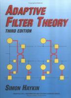
FIGURE 6.2 Distribution approximation chart for graphical solution of the Ozturk algorithm to the best-fit test. † mapped end point of 500 sample data set.

mapped as points in the U-V plane. Examples of these density functions include: Normal, Uniform, Exponential, Laplace, Logistic, Cauchy, and Extreme Value (type-1). The density functions that contain a single shape parameter get mapped as lines in the U-V plane. Each point on the line corresponds to a specific value of the shape parameter. Examples of these density functions include: Gumbel (type-2), Gamma, Pareto, Weibull, Lognormal, and K-distribution. Finally, the density functions that contain two shape parameters get mapped as multiple lines in the U-V plane. Each line corresponds to a fixed value of one shape parameter, with the points on this line corresponding to specific values of the second shape parameter. Examples of these density functions include the Beta and SU Johnson. The sample data set gets mapped as a single point in the U-V plane, and as stated earlier, the distributions that best fit the sample data are the ones located closest to this mapped point. As will be seen in the next section, the exact location of the mapping of distributions into the U-V plane depends upon the number of points in the data sample. The best way to ensure that a best-fit solution is accurately determined for any data set is to make sure that the U-V plane is filled with known distributions. By so doing, regardless of where in the plane the sample data gets mapped, one is assured that a known distribution will lie close to this point. In fact, it is for this reason that the distributions listed in Table 4.8 and Table 4.9 are used by the Ozturk Algorithm. Examination of Figure 6.2 demonstrates that almost the entire U-V plane is filled with known distributions. The algorithm could be made even more rigorous by adding distributions that cover other locations in the U-V plane. The graphical solution also enables one to get a feel for how precise the bestfit test is. In this example, the sample data gets mapped right on top of the curve © 2006 by Taylor & Francis Group, LLC

Applications

303 30

Best fit density functions Weibull Gamma Lognormal Gumbel (type-2)

25

f (x )

20 15 10 5 0

0

0.05

0.1

0.15

0.2

Variate (x)

FIGURE 6.3 Four of the five best-fit density functions to the text data set.

corresponding to the Weibull distribution. Therefore, the Weibull distribution provides a perfect fit to the data and is thus the most accurate density function for describing the data. Nevertheless, any of the five best-fit distributions provide a good fit for the data. In fact, these density functions when plotted together all look very similar (Figure 6.3). Therefore, any of the five density functions that the algorithm states best fit the data would very accurately describe the data. With experience, one will find that all of the density functions within a given region of the U-V plane look very similar when plotted. In this respect, one has some flexibility when choosing which best-fit density function to use for modeling data. In Figure 6.3, the K distribution has been omitted due to the complexity of this function. The parameters used to plot these functions were determined by the Ozturk algorithm. The equations describing these functions are listed in Tables 4.8 and 4.9. [Weibull: a ¼ 0.36E 2 3, b ¼ 0.029, g ¼ 1.3; Gamma: a ¼ 0.28E 2 2, b ¼ 0.015, g ¼ 2.0; Gamma: a ¼ 0.28E 2 2, b ¼ 0.015, g ¼ 2.0; Lognormal: a ¼ 0.022, b ¼ 0.044, g ¼ 0.41; Gumbel (type-2): a ¼ 0.64, b ¼ 0.66, g ¼ 40.] A goodness-of-fit test was also performed on these data. When doing a goodness-of-fit test, the sample data are compared with a specified distribution (the null distribution). After selecting a density function for the null distribution, values for the shape parameters must be given (if applicable). Two different null distributions were used for the goodness-of-fit test: Normal and Weibull. Since the Normal distribution lacks any shape parameters, none were specified. For the Weibull distribution, the shape parameter used for the goodness-of-fit test was 1.3 (the one found from the best-fit test). The results of these goodness-offit tests are shown in Figure 6.4. In this test the sample data and null hypothesis distribution get mapped as trajectories in the U-V plane. Based on these tests, a Normal distribution for the sample data can be rejected with 99% confidence level while a Weibull distribution can be accepted with 99% confidence level. © 2006 by Taylor & Francis Group, LLC

Adaptive Antennas and Receivers 0.4

0.4

0.35

0.35

0.3

0.3

0.25

0.25

0.2

v

v

304

0.15

(a)

0.2 0.15

0.1

0.1

0.05

0.05

0 –0.1– 0.05 0 0.05 0.1 0.15 0.2 0.25 0.3 0.35 u

(b)

0 – 0.1 –0.05 0 0.05 0.1 0.15 0.2 0.25 0.3 u

FIGURE 6.4 Comparison of two goodness-of-fit tests for the same sample data. (a) Null hypothesis distribution is normal. (b) Null hypothesis distribution is Weibull.

The outer ellipse corresponds to a 99% confidence level, middle ellipse to a 95% confidence level, and inner ellipse to a 90% confidence level. The larger the ellipse, the more likely the sample distribution will pass through the ellipse. The details of the goodness-of-fit test will be discussed in the following section. However, the basic premise of the graphical solution is that the sample data and the null distribution get mapped as trajectories in the U-V plane. To create these trajectories, the Ozturk Algorithm first generates the same number of samples from the null distribution as are present in the sample data. Next, both the sample data and the null data are ordered sequentially in ascending order. (It is for this reason that independent random data samples must be used.) Finally, each data point from the sample and null data set is converted to an ordered statistic and mapped in the U-V plane. These mapped points are connected to form the resulting trajectories, as illustrated in Figure 6.4. If the data are completely consistent with the null distribution, these two trajectories will overlap everywhere. On the other hand, if the data are not consistent with the null distribution, these two trajectories will differ considerably. As can be seen in Figure 6.4, the mapped trajectory of the data and the Normal distribution differ markedly, whereas the trajectory of the data and the Weibull distribution (for a shape parameter of 1.3) almost completely overlap. Therefore, these trajectories provide one with qualitative information regarding the goodness-of-fit test: the more identical the trajectories, the more similar are the data and the null distribution. It is important to remember, however, that for those distributions described by shape parameters, every value of the shape parameter will lead to a differently mapped trajectory. The graphical solution to the goodness-of-fit test also provides quantitative information. Confidence ellipses are plotted for the end point of the null distribution trajectory. Therefore, the center of the confidence ellipses corresponds to the end point of the mapped null distribution trajectory. Three confidence ellipses are plotted. The largest ellipse corresponds to a confidence level of 99% (0.01 level of significance), the middle ellipse to a confidence level of 95% © 2006 by Taylor & Francis Group, LLC

Applications

305

(0.05 level of significance), and the smallest ellipse to a confidence level of 90% (0.10 level of significance). The confidence ellipses describe the probability that the end point of the mapped trajectory from the sample data will lie within the ellipses given that the null distribution is true. In other words, given that the null hypothesis is true, the end point of the trajectory from the sample data will be located inside the largest ellipse 99% of the time, the middle ellipse 95% of the time, and the smallest ellipse 90% of the time. Put in another way, if the end point of the mapped trajectory from the sample data lies outside of the large ellipse, the null hypothesis can be rejected with 99% confidence (or a 0.01 level of significance). The level of significance refers to the probability that the null hypothesis is rejected given that it is true. Therefore if the mapped end point from the sample data lies outside of all the confidence ellipses, we can reject the null hypothesis with a level of significance greater than 0.01. This means that we will be wrong in rejecting the null hypothesis less than one percent of the time. In this particular example, it is evident that the Normal distribution can be rejected as the null hypothesis with 99% confidence and that the Weibull distribution is consistent with the null hypothesis with 99% confidence. It is important to point out that the size of the confidence ellipses is completely determined by the choice of the null distribution and the number of points in the sample data set. This statement is intuitively satisfying. The fewer the number of points, the larger the confidence ellipses will be. When few data points are present, the confidence ellipses will cover a large portion of the U-V plane, and almost all data sets will map inside these ellipses. This fact makes sense because if only a few samples (say, 10 to 20) are used, it is almost impossible to reject the idea that these data are from a specific density function. On the other hand, as the number of data points increases, the confidence ellipses eventually converge to a single point in the U-V plane. Therefore, in theory, a data set with an infinite number of points will be consistent with only one PDF. Similarly, the variability of the null distribution affects the size of the confidence ellipses: the greater the variability of the null distribution, the larger the confidence ellipses. One last point concerning the confidence ellipses merits mentioning. When the Ozturk Algorithm implements the graphical solution to the best-fit test, the confidence ellipses are also plotted on the distribution approximation chart. This can be seen in Figure 6.4 where the Normal distribution was specified as the null distribution. Notice that the three confidence ellipses are plotted as dotted circles around the “N” in this figure. Also notice that the U-V coordinates for the confidence ellipses in Figures 6.2 and 6.4 agree. Thus, even when doing a best-fit test, information about the goodness-of-fit test is provided by the Ozturk Algorithm. Now that a basic understanding of the Ozturk Algorithm has been presented, a detailed discussion of the best-fit test and goodness-of-fit test will be provided in the next section. Those readers who are only interested in the applications of the Ozturk Algorithm and not in the mathematical specifics of its operation may omit this section. © 2006 by Taylor & Francis Group, LLC

306

Adaptive Antennas and Receivers

6.1.2. DETAILED D ESCRIPTION OF

THE

O ZTURK A LGORITHM

In this section, a detailed explanation of how the Ozturk Algorithm performs the best-fit test and goodness-of-fit test will be given. Initially, the concept of a standardized order statistic will be discussed. Then, the technique used by the Ozturk Algorithm to perform the goodness-of-fit test will be described. This discussion will include how the sample data and null distribution get mapped as trajectories in the U-V plane and how the confidence ellipses are calculated. Finally, the technique used by the algorithm to perform the best-fit test will be discussed. A description of how the parameters in a best-fit test for a particular distribution are calculated will be given. The theoretical information in this section describing the operation of the Ozturk Algorithm has been taken from several sources (Shah,2 Ozturk,1 and Ozturk and Dudewicz4). 6.1.2.1. The Standardized Order Statistic The Ozturk Algorithm is appropriate for analyzing any unimodal random data set. Currently, the algorithm is in the process of being expanded to multivariate and multimodal distributions (personal communication). The one assumption the algorithm makes is that the random data are from independent trials, and thus, the order of the data does not matter. Data for which this assumption is not valid should not be used by the algorithm. The Ozturk Algorithm organizes the data samples in sequential order: X1, X2, X3, …, Xn, such that X1 , X2 , X3, …, , Xn. The standardized i th order statistic ðYi Þ for each sample is defined as Yi ¼ Xi 2 mx =sx ; i ¼ 1; 2; 3; …; n where

mx ¼

n X Xi n 1

is the sample mean and

sx ¼

n X i

sffiffiffiffiffiffiffiffiffiffiffiffiffiffiffi ðXi 2 mx Þ2 n21

is the sample standard deviation. One of the major advantages of the standardized order statistic is that it is invariant under linear transformation. The usefulness of this property will become evident shortly. Table 4.8 and Table 4.9 list all of the PDFs that the Ozturk Algorithm currently uses. These functions are listed both in standard form and general form, where the difference between the two is that the general form incorporates the transformation y ¼ ðx 2 aÞ=b: Therefore, as indicated in the tables, the relationship between the standard form and the general form of the PDFs is gðxÞ ¼ f ðyÞ

© 2006 by Taylor & Francis Group, LLC

dy dx

x2a y¼ b

¼

1 x2a f b b

Applications

307

In the general form of the density function, a and b are referred to as the location and scale parameters, respectively. The advantage of using standardized order statistics is that given the linear transformation described above, the standard order statistics of the random variable X and Y are equal. That is Yi 2 my X 2 mx ¼ i sy sx where mx, my, sx, and sy, are the sample means and sample standard deviations as defined previously. The above statement can easily be proven by noting that

my ¼

m E½X 2 x ¼0 sx sx

and sffiffiffiffiffiffiffiffiffiffi Var½X ¼1 sy ¼ s2x This property enables the Ozturk Algorithm to perform the goodness-of-fit test and best-fit test using the standard form of the PDFs (a simpler form than the general one). As a result, in these calculations, the location and scale parameters are irrelevant since they do not affect the standardized order statistics. Put in another way, by using the standardized order statistics, the algorithm normalizes the data for any location and scale parameter. The end result is that only the shape parameters and type of density function affect the standardized order statistics. It is for this reason — as will be seen later in this section — that density functions that lack any shape parameters map as points in the U-V plane, whereas those density functions that have either one or two shape parameters map as a line or a series of lines in the U-V plane. 6.1.2.2. The Goodness-of-Fit Test The Ozturk Algorithm has two modes of operation: a goodness-of-fit mode and a best-fit mode. A detailed description of the goodness-of-fit test will be provided first because once the procedure for this test has been explained, it will be easier to understand the best-fit test. To perform the goodness-of-fit test, the Ozturk Algorithm uses three sets of data: a reference distribution, a null distribution, and a sample data set. For convenience, in this algorithm, the standard normal distribution is used as the reference distribution. However, there is no reason that another distribution could not be used. Similarly, the null distribution may be any density function that is listed in Tables 4.8 and 4.10. Nevertheless, one should keep in mind that additional distributions could be used as the null distribution if they were programmed into the Ozturk Algorithm. In addition to specifying that density function to use as the null distribution, it is also necessary to define all values © 2006 by Taylor & Francis Group, LLC

308

Adaptive Antennas and Receivers

of the shape parameters (if applicable) for that density function. Finally, the sample data may describe any univariate random variable whose samples are independent events. The number of samples in the data set may range from 1 to 9000; however, it is recommended that one use at least 50 data points to obtain accurate results. The number of data points calculated for the reference distribution and the null distribution is the same as the number of data points in the sample data set. The idea behind the goodness-of-fit test is that all of the points in the sample data set and null distribution are ordered sequentially, and then standardized order statistics are calculated for each point. The algorithm then transforms these statistics into linked vectors, one vector for each point. The magnitude of the vectors is determined by the sample data and null distribution while the angle of the vector is determined solely from the reference distribution. The sum of these vectors leads to the mapped trajectories in the U-V plane: one for the sample data and one for the null distribution (see Figure 6.4). Confidence ellipses are then calculated for the end point of the mapped trajectory of the null distribution. 6.1.2.3. Calculation of Linked Vectors in the U-V Plane In this section the random variable X will be used when describing the sample data set, the random variable N will be used when describing the null distribution, and the random variable R will be used when describing the reference distribution. The following paragraphs explain the procedure used by the Ozturk Algorithm for computing the linked vectors. The sample data from which the standardized order statistics are calculated is entered into the algorithm as a text file. In contrast, the average of 2000 Monte Carlo simulations is used to generate data for the reference and null distribution. The number of points generated with each Monte Carlo simulation is the same as the number of samples in the data set to be analyzed. The first calculation made by the algorithm is to order each of the samples as described below: X1 ; X2 ; X3 ; …; Xn

N1;k ; N2;k ; N3;k ; …; Nn;k

R1;k ; R2;k ; R3;k ; …; Rn;k ð6:3Þ

such that X1 , X2 , X3 , · · · , Xn N1;k , N2;k , N3;k , · · · , Nn;k R1;k , R2;k , R3;k , · · · , Rn;k

ð6:4Þ

where Ni;k refers to the i th order statistic from the k th Monte Carlo trial for the null distribution and Ri;k refers to the i th order statistic from the k th Monte Carlo trial for the reference distribution. Once this ordering has been performed, the Ozturk Algorithm calculates standardized order statistics for each distribution. © 2006 by Taylor & Francis Group, LLC

Applications

309

The equations describing this process are listed below: Yi ¼ Mi ¼

Xi 2 mx ; sx

i ¼ 1; 2; 3; …; n

X ðNi Þk 2 mn;k 1 2000 ; 2000 k¼1 sn;k

Si ¼

X 1 2000 ðR Þ ; 2000 k¼1 i k

ð6:5Þ

i ¼ 1; 2; 3; …; n

i ¼ 1; 2; 3; …; n

ð6:6Þ

ð6:7Þ

where mx and sx correspond to the sample mean and sample standard deviation for the sample data set and mn;k and sn;k correspond to the sample mean and sample standard deviation for the k th Monte Carlo simulation for the null distribution. Since the reference distribution used by the Ozturk Algorithm is the Standard Normal, mr;k ¼ 0 and sr;k ¼ 1: It is for this reason that these parameters are omitted in the calculation of Si. Essentially, the equations listed above indicate that the i th standardized order statistics for the null distribution and reference distribution are calculated by taking the average of 2000 i th standardized order statistics that are generated from Monte Carlo simulations. Once the above calculations have been made, the Ozturk Algorithm computes the length and orientation of each linked vector. Two sets of linked vectors are calculated: one for the sample data and one for the null distribution. The i th linked vector in each set corresponds to the i th ordered sample in the data set. The following equations describe how the magnitude and angle of these linked vectors are determined: ai ¼

lYi l n

ð6:8Þ

bi ¼

lMi l n

ð6:9Þ

1 ðSi ui ¼ puðSi Þ; uðSi Þ ¼ pffiffiffiffi e 2p 21

2t2 2

dt

ð6:10Þ

where ai represents the lengths of the i th linked vector for the sample data, bi represents the length of the i th linked vector for the null distribution, and ui represents the orientation (measured from the horizontal axis) of the i th linked vector for both the sample data and the null distribution. Notice from these equations that only the reference distribution determines the angle of the i th linked vector, and that this angle is the same for both the sample data and the null distribution. Similarly, it is the magnitude of the i th standardized order statistic that determines the length of the i th linked vector. Now that the formulas used to calculate the linked vectors have been given, it is possible to define a U-V plane where the ordered pair Qk ¼ ðUk ; Vk Þ is © 2006 by Taylor & Francis Group, LLC

310

Adaptive Antennas and Receivers

specified as follows: U 0 ¼ V0 ¼ 0

ð6:11Þ

Uk ¼

k 1X lY lcosðui Þ; n i¼1 i

k ¼ 1; 2; 3; …; n

ð6:12Þ

Vk ¼

k 1X lY lsinðui Þ; n i¼1 i

k ¼ 1; 2; 3; …; n

ð6:13Þ

A similar ordered pair, Pk ¼ ðU0k ; V0k Þ, is likewise defined below: U00 ¼ V00 ¼ 0

ð6:14Þ

U0k ¼

k 1X lM lcosðui Þ; n i¼1 i

k ¼ 1; 2; 3; …; n

ð6:15Þ

V0k ¼

k 1X lM lsinðui Þ; n i¼1 i

k ¼ 1; 2; 3; …; n

ð6:16Þ

The first set of equations defines the trajectory of linked vectors associated with the sample data, while the second set of equations defines the trajectory of linked vectors associated with the null distribution. The Ozturk Algorithm graphs the mapped trajectories found in the goodness-of-fit test by connecting the set of points described by Qk and Pk for k ¼ 1; 2; 3; …; n: A few general comments about the above equations are worth mentioning. One important thing is to remember that the angle of the i th linked vector is purely determined by the reference distribution is the same for both the sample data and the null distribution, and based on how it is defined, starts at 0 and increases to a maximum of 180 degrees (as measured from the horizontal axis). For this reason the general shape of all of the trajectories in the goodness-of-fit test are similar (Figure 6.4). In addition, due to the definition of the standardized order statistic, the magnitude of the i th linked vector for the sample data and null distribution start out large, then decrease to almost zero, and then become large again. The length of these vectors reach a minimum around an angle of 908. It can also be seen from the above equations that Qn and Pn represent the endpoint of the linked vectors for the sample data and null distribution, respectively. Finally, the trajectories defined by Qk and Pk for k ¼ 1; 2; 3; …; n become smoother as the number of samples (n) increases. Although the Ozturk Algorithm only generates confidence ellipses for the end point of the null distribution trajectory, qualitative information about the goodness-of-fit test is provided by comparing the path of the trajectory for the sample data with that for the null distribution. It is reasonable to expect that the linked vectors from the sample data will closely follow the linked vectors from the null distribution if the sample data are consistent with the null © 2006 by Taylor & Francis Group, LLC

Applications

311

distribution. As a result, the goodness-of-fit test provides visual information about how well the ordered set of data fit the null distribution (Figure 6.4). Nevertheless, the Ozturk Algorithm also uses statistical procedures for quantifying the goodness-of-fit test through the calculation of confidence ellipses. This procedure is described next. 6.1.2.4. Calculation of Confidence Ellipses The confidence ellipses provide a quantitative statistical description of how consistent the sample data are with the null distribution. As discussed earlier, if the end point of the trajectory for the sample data ðQn Þ falls within one or more of the ellipses, the sample data set is said to be statistically consistent with the null hypothesis at a confidence level based on the confidence ellipses. Each confidence contour is directly associated with a significance level and is defined as the conditional probability that the end point of the trajectory for the sample data ðQn Þ falls inside the specified ellipse given that the data comes from the null distribution. Therefore, the 99% confidence ellipse corresponds to a 0.01 level of significance, the 95% confidence ellipse corresponds to a 0.05 level of significance, and the 90% confidence ellipse corresponds to a 0.10 level of significance. To understand how the Ozturk Algorithm calculates the confidence ellipses, one must remember that the algorithm performs 2000 Monte Carlo simulations of sample size n for the null distribution. Therefore, 2000 end points are calculated, and the average of these values is used as the actual value of the end point ðQn Þ: As a result, the endpoint ðQn Þ corresponds to the ordered pair ðU0n ; V0n Þ where both U0n and V0n are random variables consisting of 2000 samples. It is from these random variables that the confidence ellipses are calculated. The actual nature of the underlying distribution for the random variables U0n and V0n is unknown. However, if these variables were described by a bivariate Gaussian distribution, the calculation of the confidence ellipses would be straightforward. A three dimensional bell shaped Gaussian curve could be fit to the 2000 end points calculated by the Monte Carlo simulation and the corresponding confidence ellipses plotted for the desired significance levels. If a correlation existed between the random variables U0n and V0n the confidence contours would be ellipses, but if no correlation existed, the confidence contours would be circles. Unfortunately, however, as just mentioned, the underlying distributions of U0n and V0n are not known. Therefore, the Ozturk Algorithm uses a complicated procedure to transform the random variables U0n and V0n into a single random variable that is bivariate Gaussian. After this transformation is made, the confidence ellipses are calculated. Finally, the actual confidence contours are obtained by taking the inverse transform of the confidence ellipses obtained from the bivariate Gaussian random variable. A family of distributions called the Johnson System is used to perform the transformation on U0n and V0n in order to obtain a bivariate Gaussian distribution. The details of this transformation are tedious and beyond the scope of this chapter. A complete description of this process can be found in (Shah2). © 2006 by Taylor & Francis Group, LLC

312

Adaptive Antennas and Receivers

Two comments about the confidence ellipses are worth mentioning. For one thing, the confidence contours will only be ellipses if U0n and V0n can be described by a bivariate Gaussian distribution without undergoing any transformation. In all other cases, these confidence contours may not look like ellipses due to the transformation process. Hence, the phrase “confidence ellipses” is used loosely in this chapter since many of these contours are not actually ellipses. In addition, the size of the confidence ellipses depends on the sample size ðnÞ and the selection of the null distribution. As the sample size decreases, the variability in Pn increases, and the confidence ellipses become larger. Similarly, if a null distribution is selected that has a high degree of variability, the variability of Pn will also be high, and the confidence ellipses will be relatively larger (for a given sample size). If the sample size used is too small (less than 50 samples), the confidence ellipses become so large that the goodness-of-fit test becomes meaningless; almost any sample data will be consistent with the null hypothesis. Nevertheless, an inspection of the mapped trajectories between the sample data and the null distribution provides a qualitative indicator of how consistent the data and the null distribution are. 6.1.2.5. The Best-Fit Test The best-fit test uses a distribution approximation technique and is simply an extension of the goodness-of-fit test. A detailed discussion of this procedure can be found in Shah2 and Ozturk.1 In the goodness-of-fit test, it was explained how trajectories for the sample data and null distribution get mapped into the U-V plane. The ordered pairs, Qn and Pn , correspond to the end points of these trajectories. In the best-fit test, this procedure is extended one step further; the end point for every distribution is calculated and plotted in the U-V plane. In addition, since the end point for a particular distribution depends on the value of the shape parameters, for those distributions where shape parameters exist, end points for several values of these shape parameters are computed, and these end points are mapped as trajectories in the U-V plane. In other words, only one end point is calculated for those distributions that lack any shape parameters (Normal, Uniform, Exponential, Laplace, Logistic, Cauchy, and Extreme Value [type-1], and this end point maps as a point in the U-V plane; several end points are calculated for those distributions containing one shape parameter [Gumbel (type-2)], Gamma, Pareto, Weibull, Lognormal, and K-distribution), and these end points map as a line in the U-V plane; and even more end points are calculated for those distributions containing two shape parameters (Beta and SU Johnson), and these end points map as a series of lines in the U-V plane. As an example, the Ozturk Algorithm calculates end points for the Weibull distribution for the following values of the shape parameter: 0.3, 0.4, 0.5, 0.6, 0.8, 1.1, 1.5, 2.0, 3.0, and 5.0. These end points are then mapped in the U-V plane, connected and correspond to the line labeled Weibull in the distribution approximation chart (Figure 6.2). When a distribution contains two shape parameters, then the first shape parameter is held constant © 2006 by Taylor & Francis Group, LLC

Applications

313

at some value while the second shape parameter is varied, and then this process is repeated for different values of the first shape parameter. It is important to keep in mind that each end point is computed from 2000 Monte Carlo simulations where the number of samples used in the simulation ðnÞ matches the number of points in the sample data set. Therefore, the appearance of the U-V plane for the best-fit test (Figure 6.2) is dependent upon the number of samples in the data set being analyzed. Although the above process may seem very tedious and time consuming, the Ozturk Algorithm speeds up this process considerably by tabulating data. In other words, the coordinates of the end points for specific values of the shape parameters and a specific distribution are stored in a data table as a function of sample size. Using this technique, it becomes unnecessary to recalculate these end points with each simulation, which would greatly slow down the processing time. In addition, for those distributions that contain shape parameters, the Ozturk Algorithm only calculates (stores) end points for a fixed number of values for these shape parameters. These points are then connected together to form the lines in the U-V plane found in the distribution approximation chart. Once a distribution approximation chart is generated for all of the distributions stored in the algorithm’s library and for the particular sample size of the data set, the sample data is mapped in the U-V plane. Recall that the coordinates of the end point for the sample data correspond to the point, Qn : This graphical solution to the best-fit test is referred to by the Ozturk Algorithm as the Distribution Approximation Chart (Figure 6.2). Inspection of this plot allows one to determine which distributions most closely fit the data; those distributions that lie closest to the mapped data point ðQn Þ provide the best fit. In addition to this graphical solution, the Ozturk Algorithm also determines which five distributions best fit the data. The algorithm determines the closest point or trajectory by projecting the mapped data point to neighboring points or trajectories on the chart, and selecting the point or trajectory whose perpendicular distance from the sample point is the smallest. If the identified density functions contain shape parameters, the values of these parameters are determined through interpolation. One must remember that the distributions are mapped in the U-V plane by connecting the end points corresponding to selected values of the shape parameters. It should also be noted that the library of density functions has been carefully chosen such that most of the U-V plane is filled with mapped end points or trajectories of end points. In so doing, the algorithm ensures that regardless of where the end point of the sample data is mapped in the U-V plane, there will be a mapped distribution located close to this end point. After the algorithm identifies the five density functions which best fit the sample data and interpolates the value of the shape parameters (if applicable), then the standard form of the density function is completely characterized (as indicated in Tables 4.8 and 4.9). However the location (a) and scale (b) parameters still need to be computed. Recall that the Ozturk Algorithm makes use © 2006 by Taylor & Francis Group, LLC

314

Adaptive Antennas and Receivers

of standardized order statistics that are independent of linear transformations such as the location and scale parameters. Therefore, to compute the location and scale parameters, the process of taking standardized order statistics must be reversed. The process used by the algorithm to compute the value of the location and scale parameters is described next. 6.1.2.6. Estimation of Location and Scale Parameters The Ozturk Algorithm calculates the value of the location (a) and scale (b) parameters by inverting the procedure used to generate the standardized order statistics. Recall that the random variable X corresponds to the sampled order data while the random variable Y corresponds to the standardized order statistics for the sample data. The relationship between these two variables is that Yi ¼ ðXi 2 aÞ=b where Yi represents the i th standardized order statistic and Xi represents the i th sampled order data. Once the Ozturk Algorithm specifies the distributions that best fit the data along with the corresponding value of the shape parameters (if applicable), then the random variable Y is completely described according to the standard form of the density functions listed in Tables 4.8 and 4.9. In order to obtain a complete description of the random variable X, the location and scale parameters must be computed. To calculate the value of these two parameters, the algorithm defines two new variables as follows: C1 ¼ C2 ¼

n X i¼1 n X i¼1

cosðui ÞXi

ð6:17Þ

sinðui ÞXi

ð6:18Þ

where ui corresponds to the angle defined by Equation 6.10, Xi refers to the random variable describing the i th ordered sample from the data set, and n corresponds to the number of samples in the data set. Based on the definition of the above two variables and making use of the substitution E½Xi ¼ bmi þ a, the expected values of C1 and C2 are equal to: E½C1 ¼ E½C2 ¼

n X i¼1 n X i¼1

cosðui Þðbmi þ aÞ

ð6:19Þ

sinðui Þðbmi þ aÞ

ð6:20Þ

where mi represents the sample mean of Yi : The value of mi is calculated by the Ozturk Algorithm by running 2000 Monte Carlo simulations for the standard form of the best-fit density function described by Yi and averaging the means of these simulations. In other words, the algorithm uses the standard form of the selected best-fit distribution (as described in Tables 4.8 and 4.9) to generate n samples © 2006 by Taylor & Francis Group, LLC

Applications

315

from this density function, and takes the average of these samples. This process is repeated for 2000 simulations, and the average of all of these simulations is the value used for mi : The equations describing the expected values of C1 and C2 can be rewritten as: E½T1 ¼ aa þ bb

ð6:21Þ

E½T2 ¼ ca þ db

ð6:22Þ

where n X

a¼

cosðui Þ

ð6:23Þ

mi cosðui Þ

ð6:24Þ

i¼1

b¼

n X i¼1

c¼

n X

sinðui Þ

ð6:25Þ

mi sinðui Þ

ð6:26Þ

i¼1

d¼

n X i¼1

Since the standardized Gaussian distribution is used by the Ozturk Algorithm as the reference distribution, ui starts at 0 ði ¼ 1Þ and ends up at p ði ¼ nÞ: Therefore, a ¼ 0, as defined above. Rearranging the preceding equations and letting a ¼ 0, it can be shown that:

a¼

E½T2 2 d b c

ð6:27Þ

E½T1 b

ð6:28Þ

b¼

If the sample size is sufficiently large (i.e., n . 50), it can be shown that E[T1] ¼ T1 and E[T2] ¼ T2 (Shah2). In addition, since the algorithm computes the value of mi , as described above, and the value of ui is also calculated, values for the variables b; c and d are easily obtained. Using these values, the algorithm computes the value of the location and scale parameters. Once these two parameters are calculated, the general form of the density function describing the random variable X is completely defined (as indicated in Tables 4.8 and 4.9). In this section of the chapter, a detailed description of the technique used by the Ozturk Algorithm to perform a goodness-of-fit test and best-fit test was provided. In the next three sections, three applications of the Ozturk Algorithm in the field of neuroscience will be presented. © 2006 by Taylor & Francis Group, LLC

316

Adaptive Antennas and Receivers

6.1.3. ANALYSIS OF S PONTANEOUS AUDITORY N ERVE ACTIVITY OF C HINCHILLAS The usefulness of the Ozturk Algorithm for analyzing data will first be demonstrated using data from the auditory nerve. All of the data analyzed in this section was provided by Evan Relkin and was recorded from chinchillas. One of the major limitations when recording from a single unit is the ability to maintain a stable recording from an auditory fiber for an extended period of time. Nevertheless, one must make sure that enough data are collected so that an accurate analysis of these data can occur. It would be of considerable advantage to the investigator if spike trains could be recorded for a shorter amount of time for each stimulating condition without compromising the information gained from these data. In this section, it will be shown how the Ozturk Algorithm can be used to gather data more efficiently. In the first part of this study, spontaneous nerve activity was analyzed. The random variable inputted into the algorithm was the time between successive spikes (i.e., interspike intervals). Since these spike trains are undriven, they are not subjected to adaptation, and hence, they represent random, independent events. One must recall that the Ozturk Algorithm assumes the data set to consist of independent trials. For this reason, driven spike trains are not considered. Two different fibers were analyzed, one with a spontaneous activity of 38 spikes/sec (fiber #1) and one with a spontaneous activity of 74 spikes/sec (fiber #2). According to Liberman,5 both of these fibers would be classified as high spontaneous rate (SR) fibers. (Liberman classifies those fibers having an SR greater than 17.5 spikes/sec as high SR, between 0.5 and 17.5 spikes/sec as medium SR, and below 0.5 spikes/sec as low SR.) The purpose of this portion of the study was to determine the minimum number of interspike intervals necessary to accurately characterize the interspike interval histogram. In addition, the Ozturk Algorithm was used to determine how the best-fit distributions, for fibers of two different spontaneous activities, compare. For the fiber with a spontaneous activity of 38 spikes/sec (fiber #1), 2198 different interspike intervals were obtained while for the fiber with a spontaneous activity of 74 spikes/sec (fiber #2) a total of 7053 interspike intervals were collected. All of these intervals were inputted into the Ozturk Algorithm and the five best-fit distributions for each fiber were computed. Tables 6.1 and 6.2 summarize the five best-fit density functions for each fiber, respectively. For both fibers, the K-distribution provides the best fit to the data while the Gamma distribution provides the second best fit. Due to the complexity of the K-distribution (this density function involves a form of the Bessel function that is described by a series) the Gamma distribution will be used as the best-fit approximation for the interspike interval histograms of these fibers. Figure 6.5 shows the graphical solution to the best-fit test for each fiber. From this figure, it can be seen that the Gamma function, with an appropriate value for the shape parameter, provides an excellent fit to both sets of data. Thus, the Gamma distributions as described in Tables 6.1 and 6.2 will be © 2006 by Taylor & Francis Group, LLC

Applications

317

TABLE 6.1 Parameters of Five Best-Fit Distributions, Listed in Order of Best Fit, for all 2198 Samples of Interspike Intervals of Chinchilla Auditory Nerve Activity Collected from Fiber #1 Best Fit Distributions

Location Parameter (a)

Scale Parameter ðbÞ

Shape 1 Parameter ðgÞ

Shape 2 Parameter ðdÞ

K-distribution Gamma Weibull Lognormal Exponential

20.95241E-02 20.13320E-02 20.13467E-02 20.14145E-01 20.46305E-02

0.18754E-01 0.16496E-01 0.26395E-01 0.35292E-01 0.22387E-01

0.45784E-01 0.16635E-01 0.11726E-01 0.50601E-00 —

— — — — —

assumed to provide the best characterization of the interspike interval histograms for the two fibers. In Figure 6.5, the location of the mapped data set is represented in the U-V plane by a filled circle. For fiber #1 the five distributions that are located closest to the mapped data point are the K-distribution, Gamma, Weibull, Lognormal, and Exponential. For fiber #2, the five distributions that are closest to the mapped data point are the K-distribution, Gamma, Exponential, Weibull, and Lognormal. [N ¼ Normal, U ¼ Uniform, E ¼ Exponential, A ¼ Laplace, L ¼ Logistic, C ¼ Cauchy, V ¼ Extreme Value (type-1), T ¼ Gumbel (type-2), G ¼ Gamma, P ¼ Pareto, W ¼ Weibull, L ¼ Lognormal, K ¼ K-distribution. The upper five dashed lines represent Beta, and the lower nine dashed lines represent SU Johnson.] In the next portion of this analysis, subsets of points from the sample data were inputted into the algorithm to determine the minimum number of points necessary to accurately characterize the data. For fiber #1, subsets of interspike

TABLE 6.2 Parameters of Five Best-Fit Distributions, Listed in Order of Best Fit, for all 7053 Samples of Interspike Intervals of Chinchilla Auditory Nerve Activity Collected from Fiber #2 Best fit Distributions

Location Parameter ðaÞ

Scale Parameter ðbÞ

Shape 1 Parameter ðgÞ

Shape 2 Parameter ðdÞ

K-Distribution Gamma Exponential Weibull Lognormal

20.49604E-02 20.33691E-03 0.26819E-02 0.10954E-02 20.72029E-02

0.10898E-01 0.93693E-02 0.12407E-01 0.14334E-01 0.19000E-01

0.41161E-01 0.15965E-01 — 0.11495E-01 0.51858E-00

— — — — —

© 2006 by Taylor & Francis Group, LLC

318

Adaptive Antennas and Receivers 0.6

0.6

0.5

0.5

0.3 0.2 0.1

(a)

0.4

>U W KW W W G KWL K KLTK L L N GW S P G K KP PL T A G KKW P L T K W LP T W W T L T P PP PP >C

0 −0.25 −0.2 −0.15 −0.1 −0.05 0 u

V

v

v

0.4

0.3 0.2 0.1

0.05 0.1 0.15 0.2

(b)

>U W KW W W G KWL K KLTK L L N GW S P G K KP PL T A G KKW P T K W L W LP T T WL T P PP PP >C

0 −0.25 −0.2 −0.15 −0.1 −0.05 0 u

V

0.05 0.1 0.15 0.2

FIGURE 6.5 Distribution approximation charts for two data sets. (a) fiber #1 data set. (b) fiber #2 data set. † mapped end point of entire data set.

intervals containing either 500, 150, 100, 75 or 50 data points were also analyzed by the algorithm. For each of these subsets, four different sets of data were used (i.e., four sets of 500 points, four sets of 150 points, etc.). These four sets were selected such that none of the data points appeared in more than one of the four subsets. The Ozturk Algorithm was then used to determine the best-fit Gamma distribution for each of these groups. (Recall that using all of the data, the best-fit density function for both fibers was the Gamma distribution.) Figure 6.6 summarizs these results. The graphs on the left show plots of the best-fit Gamma distributions for each of the four subsets of points; the bolded line in each plot represents the best-fit Gamma distribution for all of the data points collected from fiber #1. The graphs on the right show a portion of the graphical solution to the best-fit test as determined by the Ozturk Algorithm. These graphs show where in the U-V plane each of the four subsets of data is mapped. The filled circle in these plots represents the location of the mapped end point for the entire data set. In other words, the graphs on the right show the U-V plane for the distribution approximation chart (see Figure 6.5) without actually showing where each of the distributions listed in Tables 4.8 and 4.9 gets mapped in this plane; only the location of the mapped data point for each of the four subsets, along with the location of the mapped data point for the entire data set are shown. (Recall that the mapped end point for each set of sample data corresponds to the point Qn , as defined in the previous section.) In Figure 6.6, the bolded line represents the best-fit Gamma distribution for the entire data set and the symbol “x” represents the corresponding mapped end point in the U-V plane. The parameter values were determined by the Ozturk Algorithm. Figure 6.6(a): open circles, a ¼ 20:0028, b ¼ 0:015, g ¼ 2:0; filled circles, a ¼ 0:00024, b ¼ 0:016, g ¼ 1:8; open squares, a ¼ 20:0017, b ¼ 0:016, g ¼ 1:6; filled squares, a ¼ 20:0012, b ¼ 0:018, g ¼ 1:6: Figure 6.6(b): open circles, a ¼ 20:0033, b ¼ 0:016, g ¼ 1:8; filled circles, a ¼ 20:00055, b ¼ 0:013, g ¼ 1:9; open squares, a ¼ 20:0019, b ¼ 0:012, g ¼ 1:9; filled squares, a ¼ 20:0029, b ¼ 0:019, g ¼ 1:7: Figure 6.6(c): open circles, © 2006 by Taylor & Francis Group, LLC

Applications

319 Best fit gamma distribution (500 points)

35

0.6

30

0.5 0.4

20

v

f (t)

25

15

0.1

5

(a)

0

0.02

0.04

0.06

0.08

0

0.1

Best fit gamma distribution (150 points)

0.6

v

f (t)

0.1

0.2

Mapped end points (150 samples)

0.4

20 15

0.3 0.2

10

0.1

5 0

0

0.5

25

0

0.02

0.04

0.06 0.08

0.1

0

–0.2

– 0.1

Time (sec)

0.6

30

0.1

0.2

Mapped end points (100 samples)

0.5

25

0.4 v

20 15

0.3 0.2

10

0.1

5 0

0 u

Best fit gamma distribution (100 points)

35

f (t)

–0.1 u

30

(c)

– 0.2

Time (sec)

35

(b)

0.3 0.2

10

0

Mapped end points (500 samples)

0

0.02

0.04 0.06 Time (sec)

0.08

0.1

0

– 0.2

– 0.1

0

0.1

0.2

u

FIGURE 6.6 Best-fit gamma distributions and mapped end points for fiber #1 interspike intervals. Distributions are shown for entire data set of 2198 samples and also for four subsets. (a) 500 samples in subset. (b) 150 samples in subset. (c) 100 samples in subset. (d) 75 samples in subset. (e) 50 samples in subset. © 2006 by Taylor & Francis Group, LLC

320

Adaptive Antennas and Receivers Best fit gamma distribution (75 points)

35

Mapped end points (75 samples) 0.6

30

0.5 0.4

20

v

f (t)

25

15 10

0.2

5

0.1

0

0

0.02

(d)

0.04

0.06

0.08

0 –0.2

0.1

– 0.1

0

Time (sec)

0.6

0.4

60

v

f (t)

Mapped end points (50 samples)

0.5

80

40

0.3 0.2

20 0

0.2

0.1

u

Best fit gamma distribution (50 points)

100

(e)

0.3

0.1 0

0.02

0.04 0.06 0.08 Time (sec)

0.1

0

– 0.2

– 0.1

0

0.1

0.2

u

FIGURE 6.6 Continued.

a ¼ 20:003329, b ¼ 0:0155, g ¼ 2:0; filled circles, a ¼ 0:0011, b ¼ 0:017, g ¼ 1:4; open squares, a ¼ 20:0021, b ¼ 0:017, g ¼ 1:8; filled squares, a ¼ 0:0050, b ¼ 0:030, g ¼ 0:79: Figure 6.6(d): open circles, a ¼ 20:0017, b ¼ 0:014, g ¼ 1:9; filled circles, a ¼ 20:0070, b ¼ 0:0090, g ¼ 3:4; open squares, a ¼ 0:0012, b ¼ 0:018, g ¼ 1:6; filled squares, a ¼ 20:0032, b ¼ 0:014, g ¼ 2:2: Figure 6.6(e): open circles, a ¼ 20:0013, b ¼ 0:014, g ¼ 2:0; filled circles, a ¼ 20:0043, b ¼ 0:021, g ¼ 0:80; open squares, a ¼ 0:0019, b ¼ 0:021, g ¼ 1:3; filled squares, a ¼ 20:0025, b ¼ 0:015, g ¼ 1:9: Inspection of Figure 6.6 qualitatively reveals that the Ozturk Algorithm does a reasonable job approximating the interspike interval histograms with as few as 50 samples. The plots of the mapped end points indicate that the variability in the location of the mapped data point when 150 samples or more are used is extremely small. However, even when as few as 50 samples are used, the location of the mapped subsets are all scattered close to the location of the mapped end point for the entire data set. The graphs of the best-fit Gamma © 2006 by Taylor & Francis Group, LLC

Applications

321

0.4

0.4

0.35

0.35

0.3

0.3

0.25

0.25

0.2

v

v

distributions are even more compelling. For all but two of the data sets (filled squares with 100 samples and filled circles with 50 samples) the best-fit Gamma distributions almost overlay exactly with the best-fit Gamma distribution for the entire data set, and even the two data sets that deviate the most only differ in a small portion of the function; the tails of these distributions all overlap. Therefore, even without any quantitative analysis, these figures indicate that 50 to 100 samples are sufficient for characterizing interspike interval histograms. Nevertheless, a goodness-of-fit test was also performed with the Ozturk Algorithm for each subset of data using the best-fit Gamma distribution for the entire data set as the null distribution, and in every case the subset of points was statistically consistent with the null distribution with a 99% confidence level. Figure 6.7 shows the graphical solution for four of these goodness-of-fit tests, two using 500 points and two using 100 points. In all four cases, the trajectory for the sample data closely follows the trajectory for the null distribution. Also notice, as explained in the previous section, that the confidence ellipses are larger when fewer samples are used. A similar analysis was also done for fiber #2; however, since this data set consists of more than 7000 interspike intervals, subsets containing 1000, 500,

0.15 0.1

0.1

0.05

0.05

0 – 0.1 – 0.05 0

0 – 0.1 – 0.05 0

0.05 0.1 0.15 0.2 0.25 0.3

0.4

0.4

0.35

0.35

0.3

0.3

0.25

0.25

0.2 0.15

0.2 0.15

0.1

0.1

0.05

0.05

0 − 0.15 −0.1−0.05 0 0.05 0.1 0.15 0.2 0.25 0.3 u

0.05 0.1 0.15 0.2 0.25 0.3 u

u

v

v

(a)

(b)

0.2 0.15

0 − 0.15 −0.1− 0.05 0 0.05 0.1 0.15 0.2 0.25 0.3 u

FIGURE 6.7 Goodness-of-fit tests for fiber #1 interspike intervals. Null hypothesis is bestfit gamma distribution for entire data set (i.e., g ¼ 1.66). Outer, middle, and inner ellipses correspond to confidence Levels of 99%, 95%, and 90%, respectively. (a) Two subsets of 500 samples. (b) Two subsets of 100 samples. © 2006 by Taylor & Francis Group, LLC

322

Adaptive Antennas and Receivers

150, 100, 75 and 50 samples were used. As before, four groups of randomly selected interspike intervals for each sample size were analyzed, except for the 1000 point case where seven data sets were used. The results of these simulations by the Ozturk Algorithm are summarized in Figure 6.8(a) to (f) and are very similar to the results from the first fiber. Once again, these graphs indicate that 50 to 100 interspike intervals are sufficient for characterizing the interspike interval histogram. The Ozturk Algorithm was also used to perform a goodness-of-fit test for each subset where the best-fit Gamma distribution for the entire data set was used as the null distribution, and once again, every subset of data was statistically consistent with the null hypothesis with a 99% confidence level. In Figure 6.8, the bolded line represents the best-fit Gamma distribution for the entire data set and the symbol “x” represents the corresponding mapped end point in the U-V plane. The parameter values were determined by the Ozturk Algorithm. Figure 6.8(a): open circles, a ¼ 2 0.00065, b ¼ 0.0091, g ¼ 1.7; filled circles, a ¼ 2 0.00021, b ¼ 0.0088, g ¼ 1.5; open squares, a ¼ 0.000079, b ¼ 0.0087, g ¼ 1.6; filled squares, a ¼ 0.00046, b ¼ 0.0085, g ¼ 1.5; open triangles, a ¼ 0.00023, b ¼ 0.0086, g ¼ 1.4; filled triangles, a ¼ 2 0.00068, b ¼ 0.0086, g ¼ 1.7; open diamonds, a ¼ 2 0.00073, b ¼ 0.0077, g ¼ 1.8; Figure 6.8(b): open circles, a ¼ 2 0.0091, b ¼ 0.0079, g ¼ 1.8; filled circles, a ¼ 2 0.00029, b ¼ 0.0072, g ¼ 1.8; open squares, a ¼ 2 0.00046, b ¼ 0.0074, g ¼ 1.7; filled squares, a ¼ 2 0.00034, b ¼ 0.0068, g ¼ 1.8. Figure 6.8(c): open circles, a ¼ 2 0.0070, b ¼ 0.0057, g ¼ 3.8; filled circles, a ¼ 0.0011, b ¼ 0.017, g ¼ 1.4; open squares, a ¼ 2 0.0021, b ¼ 0.017, g ¼ 1.8; filled squares, a ¼ 0.0050, b ¼ 0.030, g ¼ 0.79. Figure 6.8(d): open circles, a ¼ 2 0.0011, b ¼ 0.0087, g ¼ 1.3; filled circles, a ¼ 0.0039, b ¼ 0.013, g ¼ 0.75; open squares, a ¼ 0.0015, b ¼ 0.010, g ¼ 1.3; filled squares a ¼ 0.0019, b ¼ 0.0073, g ¼ 2.3. Figure 6.8(e): open circles, a ¼ 0.0036, b ¼ 0.015, g ¼ 0.77; filled circles, a ¼ 0.0028, b ¼ 0.018, g ¼ 0.88; open squares, a ¼ 0.00048, b ¼ 0.0072, g ¼ 1.5; filled squares, a ¼ 2 0.00088, b ¼ 0.0050, g ¼ 2.5. Figure 6.8(f): open circles, a ¼ 2 0.019, b ¼ 0.0019, g ¼ 16; filled circles, a ¼ 2 0.0033, b ¼ 0.0062, g ¼ 2.8; open squares, a ¼ 0.0048, b ¼ 0.0089, g ¼ 0.37; filled squares, a ¼ 2 0.0017, b ¼ 0.0039, g ¼ 3.4. In this portion of the study, the question addressed was how many samples are required to adequately produce an interspike interval histogram. The above results indicate that 50 to 100 interspike intervals are sufficient for characterizing the histogram. Furthermore, one should keep in mind that once the best-fit density function is determined, a great deal of additional information (e.g., mean and variance) also becomes available. In the next portion of this study, the Ozturk Algorithm was used to compare the best-fit density function for these two fibers. Since the spontaneous activity of these fibers differs by a factor of 2 (38 spikes/s for fiber #1 and 74 spikes/s for fiber #2) it will be interesting to see whether a single family of distributions with specific shape parameters can describe the interspike interval histogram for both fibers. © 2006 by Taylor & Francis Group, LLC

Applications Best fit gamma distribution (1000 points)

60

0.6

50

0.5

40

0.4

30

0.3

v

f (t)

323

20

0.2

10

0.1

0

(a)

0

0.02

0.04 0.06 Time (sec)

0.08

0

0.1

0.6

60

v

f (t)

30

0.2

10

0.1 0

0.02

0.04 0.06 0.08 Time (sec)

0

0.1

0.6

60

Mapped end points (500 samples)

– 0.2

–0.1

0

0.1

0.2

Mapped end points (150 samples)

0.5

50

0.4

40 v

f (t)

0.2

u

Best fit gamma distribution (150 points)

70

30

0.3 0.2

20

0.1

10

(c)

0.1

0.3

20

0

0

0.4

40

(b)

− 0.1

0.5

50

0

− 0.2

u

Best fit gamma distribution (500 points)

70

Mapped end points (1000 samples)

0

0.02

0.04 0.06 Time (sec)

0.08

0.1

0

− 0.2

− 0.1

u

0

0.1

0.2

FIGURE 6.8 Best-fit gamma distributions and mapped end points for fiber #2 interspike intervals. Distributions are shown for entire data set of 7053 samples and four subsets. (a) 1000 samples in subset. (b) 500 samples in subset. (c) 150 samples in subset. (d) 100 samples in subset. (e) 75 samples in subset. (f) 50 samples in subset.

© 2006 by Taylor & Francis Group, LLC

324

Adaptive Antennas and Receivers Best fit gamma distribution (100 points)

250

0.6 0.5 0.4

150 v

f (t)

200

100

(d)

0.1 0

0.02

0.04 0.06 Time (sec)

0.08

0

0.1

0.6

120

v

f (x)

60

0.2

Mapped end points (75 samples)

0.3

0.1

20 0

0.02

0.04 0.06 Time (sec)

0.08

0

0.1

−0.2

0

−0.1

0.1

0.2

u

Best fit gamma distribution (50 points)

70

0.6

60

Mapped end points (50 samples)

0.5

50

0.4

40 v

f (x)

0.1

0.2

40

30

0.3

20

0.2

10

0.1

0

0

0.4

80

0

− 0.1

0.5

100

(e)

− 0.2

u

Best fit gamma distribution (75 points)

140

(f)

0.3 0.2

50 0

Mapped end points (100 samples)

0

0.02

0.04

0.06

Time (sec)

FIGURE 6.8 Continued.

© 2006 by Taylor & Francis Group, LLC

0.08

0.1

0

−0.2

0

−0.1

u

0.1

0.2

Applications

325

6.1.3.1. Analysis of Two Fibers with Different Spontaneous Rates In the first part of this study, it was shown that 50 to 100 samples are sufficient for characterizing an interspike interval histogram, and that the best-fit density function is the Gamma distribution. The bottom-right graph in Figure 6.9 demonstrates how well the best-fit Gamma distribution describes binned data for 1000 interspike intervals from fiber #2. However, one interesting finding from this study was that the best-fit density function for both fibers #1 and #2 was the Gamma distribution despite the fact that the spontaneous activity of these fibers differs considerably (38 spikes/s as compared to 74 spikes/s). Therefore, one question that arises is whether a single type of density function with fixed Best fit gamma distribution (all data)

50

0.5

40

0.4

30

0.3

20

0.2

10

0.1

0

(a) 0.35

0

0.02

0.04 0.06 0.08 Time (sec)

0.1

0

−0.2

(b)

v

0.2 0.15 0.1 0.05

0.1

0.2

Histogram fitting 60 50

Frequency

0.25

0

−0.1

u

Goodness of fit test

0.3

(c)

Mapped end points (all data)

0.6

v

f (x)

60

40 30 20 10

0 0 − 0.01 − 0.1− 0.05 0 0.05 0.1 0.15 0.2 0.25 0.3 (d) u

0 0.01 0.02 0.03 0.04 0.05 0.06 0.07 0.08 0.09

Magnitude

FIGURE 6.9 Comparison of best-fit tests of sampled interspike intervals for two fibers with different spontaneous activity rates. (a) Best-fit gamma distributions for fiber #1 (filled circles) and fiber #2 (open circles). (b) Overlapping mapped end points for fiber #1 (filled circles) and fiber #2 (open circle). (c) Goodness-of-fit test for best-fit gamma distribution of fiber #1. Null hypothesis is best-fit gamma distribution of fiber #2. (d) Bestfit gamma distribution and histogram for 1000 data samples of fiber #2. © 2006 by Taylor & Francis Group, LLC

326

Adaptive Antennas and Receivers

shape parameter values can describe the spontaneous activity of any auditory nerve fiber. Using the Ozturk Algorithm, it is possible to address this question. Figure 6.9 provides some compelling evidence suggesting that the spontaneous activity for these two auditory nerve fibers is well described by a Gamma distribution with a shape parameter of approximately 1.63; the two high-SR fibers only differ in their values of the location ðaÞ and scale parameters ðbÞ: Figure 6.9(a) shows a plot of the best-fit Gamma distribution, as listed in Tables 6.1 and 6.2, for fiber #1 (filled circles) and fiber #2 (open circles). The difference between these two functions reflects the fact that fiber #2 has a spontaneous rate approximately twice that of fiber #1. However, Figure 6.9(b) shows that the data set for both of these fibers gets mapped in the same location of the U-V plane. Therefore, even though the spontaneous activity of these two fibers is different, the same type of Gamma distribution provides the best fit for both sets of data; only the values of the location and scale parameters differ. In addition, when a goodness-of-fit test is performed using the best-fit Gamma distribution for fiber #2 as the null distribution and the interspike intervals for fiber #1 as the sample data, the results indicate that the two sets of data agree almost perfectly. Figure 6.9(c) shows the graphical solution of this goodness-offit test; the sample data are statistically consistent with the null hypothesis at a 99% confidence level, and even more remarkably, the two mapped trajectories overlay almost entirely. This result provides strong evidence that, at least for these two fibers, a Gamma distribution with a shape parameter of 1.63 characterizes the interspike intervals of spontaneous auditory nerve activity. To more rigorously test this idea, an additional simulation was performed. Generally, the mathematical function thought to describe spontaneous spike generation in the auditory nerve is a Poisson process with recovery time. Therefore, a computer program was made to simulate spike generation from this process. The computer program was provided by Evan Relkin, and the recovery function used is one that was described by Gaumond et al.6,7 The simulation was run for 50 seconds using a spontaneous activity rate of 45 spikes/sec (also corresponding to a high spontaneous rate fiber). From this simulation, 2129 interspike intervals were generated. These data were analyzed by the Ozturk Algorithm, and the best-fit density function was determined to be a Gamma distribution. More remarkably, however, was the fact that the location of the mapped end point in the U-V plane was extremely similar to that for the other two fibers. In addition, when a goodness-of-fit test was performed on these data using the best-fit Gamma distribution for fiber #2 as the null distribution, the two mapped trajectories for the sample data and null data matched almost perfectly; the simulated data were statistically consistent with the null distribution at a 99% confidence level. A summary of these results is given in Figure 6.10. Although the spontaneous activity from different classifications of several more auditory nerve fibers and simulations (i.e., medium and low SR fibers) needs to be tested before definitive conclusions may be reached, the above examples demonstrate the usefulness of the Ozturk Algorithm. For one thing, the algorithm determined that a Gamma distribution with a shape parameter of © 2006 by Taylor & Francis Group, LLC

Applications

327

0.6

0.35

Fiber #1 Fiber #2 Simulation

0.5

0.3 0.25

(a)

0.2

0.3

v

v

0.4

0.15

0.2

0.1

0.1

0.05

0

− 0.2

− 0.1

0 u

0.1

0.2

(b)

0 − 0.1−0.05 0 0.05 0.1 0.15 0.2 0.25 0.3 u

FIGURE 6.10 Computer simulation of 2129 interspike intervals from a poisson process with a Gaumond recovery function. (a) Mapped end points of simulation data and entire data sets of fibers #1 and #2. (b) Goodness-of-fit test for computer simulation. Null hypothesis is fiber #2 best-fit Gamma distribution with parameters a ¼ 0.0013, b ¼ 0:016, g ¼ 1:5:

approximately 1.63 provides an excellent fit to interspike interval histograms for high-SR fibers. Secondly, the algorithm provides a method for testing the hypothesis that the spontaneous activity of all auditory nerve fibers can be described by this function. Thirdly, the Ozturk Algorithm allows a statistical verification of Gaumond’s prediction that spontaneous activity in auditory fibers can be simulated using a Poisson process with a Gaumond recovery function. Based on the above simulation, his prediction appears to be an accurate one. And lastly, the algorithm enables an even more general test of spontaneous activity to be performed. Perhaps the spontaneous rate of all types of neurons can be characterized by the same function. A similar analysis to the above one performed on different classes of neurons would provide a method for addressing this question. 6.1.3.2. Analysis of Pulse-Number Distributions The last part of the analysis in this section was done at the request of Evan Relkin. One method for analyzing spikes is to generate pulse-number distributions. In this analysis, the number of events (in this case spikes) are counted for a specific time interval, and these counts are binned for successive sweeps of the same stimulating condition (e.g., Relkin and Pelli8). Dr. Relkin is currently analyzing some data using this technique (personal communication). In his study, a 25 msec interval is used for generating the pulsenumber distributions. From these data, means and variances are computed. One problem arising with these calculations is that many more samples are required to accurately compute the variance than the mean; experimental evidence suggests that approximately the square number of samples are needed to compute the © 2006 by Taylor & Francis Group, LLC

328

Adaptive Antennas and Receivers

variance with the same accuracy as the mean. To circumvent this difficulty, Dr. Relkin has generated an equation that relates mean and standard deviation for 25 msec intervals: s ¼ 0.18m 0.36 where s corresponds to the standard deviation and m corresponds to the mean. Since the Ozturk Algorithm determines the distribution of best-fit for a set of data, and the mean and variance of these distributions are known (see Table 6.320 – 24), it was believed that the algorithm might provide a more efficient method for determining the variance of the pulsenumber distributions. The same two fibers were used in this study, and, as before, the data were provided by Evan Relkin. The stimulus paradigm was such that each stimulus condition contained 20 sweeps, and each sweep consisted of 200 ms of spontaneous activity. Pulse-number distributions were generated by counting the number of spontaneous spikes occurring in a 25 ms period. Therefore, one stimulus condition, consisting of 20 sweeps, contains 160 intervals of 25 ms. The number of 25 ms intervals used to bin the data was either 960, 500, 250, 200, 150, 100, 75, 50, or 25. For the case where 960 intervals were used, exactly six stimulus conditions of 20 sweeps were required. The Ozturk Algorithm was used to analyze these data. The random variable inputted into the algorithm was the number of spikes occurring in 25 ms interval. In other words, if 250 intervals were used, then a data set containing 250 samples was entered into the algorithm, the value of each sample representing the number of spikes that occurred in a particular 25 ms interval. It is important to point out that this random variable is discrete. Nevertheless, since the algorithm is being used to predict means and variances, as opposed to curve fitting the data, a discrete random variable is acceptable. For both fibers, nine different sets of data, each generated from a different number of samples, were analyzed. The Ozturk Algorithm was used to determine the best-fit density function for each data set. The means and variances for these distributions were computed. The formulas used for these calculations are listed in Table 6.3 and correspond to the general form of the density functions in Tables 4.8 and 4.9. One should remember that the actual class of the best-fit distribution is unimportant; it is only used to compute the means and variances. Tables 6.4 and 6.5 summarize the results obtained for fibers #1 and #2, respectively. The standard deviations were calculated by taking the square root of the variance. When the means and standard deviations generated from the Ozturk Algorithm are compared to the best-fit equation determined by Dr. Relkin, the results are impressive. Figure 6.11(a) shows these results. Although the variability around the curve is greater for the second fiber than the first one, this finding is not unusual. Dr. Relkin noticed when he was generating his curve fit that the variability around this curve increased considerably as the spontaneous rate of the fiber increased (personal communication). In fact, Dr. Relkin commented that the variability of the data from the Ozturk Algorithm was much less than the variability he normally observes. © 2006 by Taylor & Francis Group, LLC

Applications

329

TABLE 6.3 Mean and Variance of Standard and General Forms of PDFs in Tables 4.8 and 4.9 Distribution 1. Normal 2. Uniform 3. Exponential 4. Laplace 5. Logistic 6. Cauchy 7. Extreme Value (type-1) 8. Gumbel (type-2)

9. Gamma

Mean

Variance

a

b2

2a þ b 2

b2 12

aþb

b2

a

2b2

a

ðbpÞ2 3

not defined

not defined

a þ bG 0 ð1Þ where G 0 ð1Þ ¼ 20:57721 ðbpÞ2 6 G ð1 2 g 2 1Þ þ a

b2 G ð1 2 2g 2 1Þ þ 2aðb 2 1ÞG ð1 2 g21 Þ 2 G 2 ð1 2 g21 Þ

bG þ a

b2 g "

10. Pareto

bg þ ag . 1 g21

11. Weibull

bG

12. Lognormal

b exp

13. K-Distribution

1:77bG ðg þ 0:5Þ þa G ðg Þ

b2 4g 2 3:14

14. Beta

bg þa gþd

b2 gd ðg þ dÞ2 ðg þ d þ 1Þ

15. Johnson SU

gþ1 þa g g2 2

b exp

1 2g2

b2

g g 2 g22 g21

"

b2 G

sin hðdÞ þ a

# , g.2

2

gþ2 gþ1 2 G g g 2

þa

2

#

2

b2 expðg Þ ðexpðg Þ 2 1Þ "

b2 exp 2

1 g2

G ðg þ 0:5Þ G ðgÞ

2 1 exp

1 g2

2

#

cos hð2dÞ þ 1

Note: The means and variances listed above correspond to the general form of the PDFs listed in Table 4.9.

© 2006 by Taylor & Francis Group, LLC

330

© 2006 by Taylor & Francis Group, LLC

TABLE 6.4 Parameters of Best-Fit Distributions for Nine Sets of 25 msec Samples of Interspike Intervals of Chinchilla Auditory Nerve Activity Collected from Fiber #1 Number of Samples

Location Parameter ðaÞ

Scale Parameter ðbÞ

Shape 1 Parameter ðgÞ

Shape 2 Parameter ðdÞ

Distribution Mean

Distribution Std. Deviation

Beta Beta Weibull Weibull Weibull Beta Weibull Johnson S.U. Beta

960 500 250 200 150 100 75 50 25

20.71743E þ 00 20.64751E þ 00 20.21597E þ 01 20.11257E þ 01 20.16792E þ 01 20.28112E þ 00 20.2314E þ 01 0.89717E þ 00 20.63365E þ 00

0.29501E þ 01 0.28556E þ 01 0.32E þ 01 0.21774E þ 01 0.27022E þ 01 0.21496E þ 01 0.33584E þ 01 0.75416E þ 00 0.21895E þ 01

0.15966E þ 01 0.14932E þ 01 0.47862E þ 01 0.26765E þ 01 0.3746E þ 01 0.66257E þ 00 0.5E þ 01 0.12942E þ 01 0.11252E þ 01

0.16E þ 01 0.16E þ 01 — — — 0.8E þ 00 — 0 0.8E þ 00

0.75605 0.73099 0.77016 0.81068 0.75954 0.69269 0.76958 0.89717 0.64602

0.72004 0.70530 0.70162 0.77958 0.73041 0.68188 0.70625 0.80883 0.63089

Adaptive Antennas and Receivers

Best-Fit Distribution

Applications

© 2006 by Taylor & Francis Group, LLC

TABLE 6.5 Parameters of Best-Fit Distributions for Nine Sets of 25 msec Samples of Interspike Intervals of Chinchilla Auditory Nerve Activity Collected from Fiber #2 Best-Fit Distribution Beta Beta Beta Lognormal Beta Beta Beta Beta Beta

Number of Samples

Location Parameter ðaÞ

Scale Parameter ðbÞ

Shape 1 Parameter ðgÞ

Shape 2 Parameter ðdÞ

Distribution Mean

Distribution Std. Deviation

960 500 250 200 150 100 75 50 25

20.70106E þ 00 20.69648E þ 01 0.80749E þ 01 20.20146E þ 02 0.28177E þ 00 0.42671E þ 00 0.61713E þ 00 20.22230E þ 01 20.25382E þ 00

0.53329E þ 01 0.37508E þ 01 0.37225E þ 01 0.21955E þ 02 0.36410E þ 01 0.29290E þ 01 0.27104E þ 01 0.65131E þ 01 0.54295E þ 01

0.25861E þ 01 0.13357E þ 01 0.10714E þ 01 0.53507E þ 01 0.92656E þ 00 0.57095E þ 00 0.44209E þ 00 0.47614E þ 01 0.17489E þ 01

0.32E þ 01 0.16E þ 01 0.16E þ 01 — 0.16E þ 01 0.8E þ 00 0.8E þ 00 0.32E þ 01 0.32E þ 01

1.6825 1.6369 1.5737 1.8405 1.6170 1.6465 1.5818 1.6722 1.6649

1.0178 0.94149 0.95217 1.1773 0.93436 0.93774 0.86667 1.0667 1.0641

331

332

Adaptive Antennas and Receivers 1.5 Standard deviation

Standard deviation

1.5

1

0.5

0

(a)

0

y=0.81(x^0.36) Fiber #1 Fiber #2 0.5

1

1.5 Mean

2

2.5

3

0

Kaleidagraph statistic

Kaleidagraph statistic

y=0.81(x^0.36) Fiber #1 Fiber #2 0

0.5

1

1.5 Mean

2

2.5

3

2

0.8 0.6 0.4 0.2 0

0.5

(b)

1

(c)

1

0

Mean Variance 0.2

0.4 0.6 Ozturk statistic

0.8

1

1.5 1 0.5 0

(d)

Mean Variance 0

0.5

1 1.5 Ozturk statistic

2

FIGURE 6.11 Comparison of the Ozturk statistics and the sample statistics generated by Kaleidagraph application. (a) Ozturk statistics vs. curve fit determined by Evan Relkin. (b) Kaleidagraph statistics vs. curve fit determined by Evan Relkin. (c) Ozturk statistics vs. Kaleidagraph statistics for fiber #1. The line in this graph passes through the origin and has a slope of one. (d) Ozturk statistics vs. Kaleidagraph statistics for fiber #2. The line in this graph passes through the origin and has a slope of one.

The application, Kaleidagraph, was also used to calculate sample means and standard deviations for all of the data inputted into the Ozturk Algorithm. These data are shown in Figure 6.11(b). It is interesting to note that unlike the statistics generated from the Ozturk Algorithm, all of the sample statistics fall on one side of the curve (with the exception of one data point from fiber #2). In fact, when calculating the deviation of the Ozturk statistics and Kaleidagraph statistics from Evan Relkin’s curve fit, it was found that the mean-square deviation of the Ozturk statistics was 9% less for fiber #1 and 18% less for fiber #2 than the deviation for the corresponding Kaleidagraph statistics. Another way to compare the two methods for calculating statistics is to plot the Ozturk mean and variance versus the sample mean and variance for each set of data.† Figure 6.11(c) and (d) shows this comparison. The line drawn in these

†

The variance has been plotted instead of the standard deviation since the mean and standard deviation for fiber #1 are similar, and thus, the data points would overlay in this plot.

© 2006 by Taylor & Francis Group, LLC

Applications

333

graphs passes through the origin and has unity slope. If the statistics from both methods matched perfectly, one would predict that the data would fall on this line. As can be seen from these graphs, for fiber #1, the Kaleidagraph statistics for both mean and variance are consistently greater than those of the Ozturk statistics; for fiber #2, although the sample mean and Ozturk mean agree well, the sample variance is consistently greater than the Ozturk variance. Therefore, by using the Ozturk Algorithm to determine the distribution of best-fit and calculating the mean and variance of this distribution, one obtains a more accurate prediction of these statistics than by using the sample statistics. In addition, it is important to keep in mind that the Ozturk Algorithm can generate an excellent estimate of the pulse-number distribution’s mean and variance with as few as 25 samples.

6.1.4. ANALYSIS o F E FFERENT O PTIC-N ERVE ACTIVITY IN THE H ORSESHOE C RAB The second application of the Ozturk Algorithm was analyzing efferent optic nerve activity in the horseshoe crab. Numerous studies have been carried out to demonstrate the effects of the efferent activity on visual sensitivity. Some of these studies include Barlow et al.9, Kass and Barlow10, Chamberlain and Barlow11,12, Barlow et al.13, and Kier and Chamberlain.14 Two additional studies provide a detailed description of the organization of the efferent activity (Barlow15 and Kass and Barlow16). Some of the conclusions from these two studies include: 1. Each lateral optic nerve contains a small but separate group of efferent fibers (approximately 10 to 20). 2. Efferent fibers fire in bursts at rates up to two bursts per second. 3. Each efferent fiber fires one spike in a burst. 4. Bursts occur synchronously in the lateral optic nerves. 5. Efferent activity undergoes a circadian rhythm. 6. Coupling among efferent neurons changes during the circadian cycle. Although several effects of the efferent activity on visual sensitivity are known and some general properties about the organization of this activity have been made, a detailed study of the structure of this information was lacking. For example, Barlow15 comments, “The repetitive bursts of impulses indicate that the efferent cell bodies in the brain are either coupled together or receive nearly synchronous inputs from the circadian clock. The bursts become less distinct in the early morning hours, suggesting that the synchrony changes during the circadian cycle.” In other words, Barlow observed that the efferent activity occurred in bursts, with each fiber firing once per burst, and that these bursts slowed down at dusk (onset of activity) and dawn (offset of activity) and were most rapid in the middle of the night. To further explore the organization of the efferent activity, Chris Passaglia and I performed an additional study (Passaglia et al.17). In this study, we found a © 2006 by Taylor & Francis Group, LLC

334

Adaptive Antennas and Receivers

patterned structure to the activity; bursts of spikes occur in clusters, and these clusters of bursts occur in packets. In general, the time between bursts is less than ten seconds, the time between clusters is around ten seconds, and the time between packets is on the order of minutes. Figure 6.12 illustrates these concepts by showing several minutes of efferent activity throughout the night. Each “spike” in these traces correspond to a burst of action potentials. We also observed in our study that the efferent activity was highest in the middle of the night, and that the time between bursts, clusters, and packets all increased at the onset and offset of activity. In other words, the efferent activity started off slowly (long time between bursts, clusters, and packets) increased to its fastest rate during the middle of the night, and then gradually slowed down again toward morning. During the day there is no efferent activity. Figure 6.12 also illustrates this phenomenon. To help learn about the structure of the efferent activity, the Ozturk Algorithm was used to analyze the best-fit distributions for the interburst intervals. In Figure 6.12, there was no activity recorded before 6 p.m. or after 6 a.m. in this animal, and the activity was most rapid between 11 p.m. and 1 a.m. Each spike in these traces corresponds to a burst of action potentials, and each efferent fiber fires one action potential per burst. The upper-left inset shows an expanded time scale where approximately seven action potentials can be resolved.

6 pm

Burst

0.2 sec

7 pm

9 pm

11 pm

Cluster

Packet

1 am

3 am

5 am

6 am

10 sec

FIGURE 6.12 Eight 3-min traces of horseshoe crab efferent optic nerve activity recorded throughout the night. © 2006 by Taylor & Francis Group, LLC

Applications

335

The number of action potentials occurring in each burst stays constant throughout an experiment. 6.1.4.1. Characterization of Interburst Intervals Given the observation that the rate of the efferent activity is modulated throughout the night, an interesting question that arises is whether a single distribution can provide a good fit to the data regardless of the time of the activity. In other words, as the efferent activity is modulated, does the type of distribution which best fits the data change, or rather does the best-fit distribution remain the same and the parameters of this distribution change? Since the Ozturk Algorithm assumes independent samples, only interburst intervals, and not the time between clusters and packets, were analyzed. In addition, data samples were only analyzed over a maximum duration of a one hour interval, the assumption being that the efferent spike trains remain relatively stationary over this interval, and hence, the assumption of independent trials remains valid. Qualitative inspection of the efferent spike trains over one hour intervals supports this assumption. The efferent spike trains that were recorded from these intervals included the time of occurrence of all of the spikes. The data were transformed into interspike intervals by calculating the time between successive spikes. Intervals corresponding to times between clusters and packets were subjectively identified and deleted. Three experiments, done on three different animals, were analyzed. For each of these experiments, the interburst data for successive one hour intervals were analyzed. For all three experiments, the Ozturk Algorithm was used to determine the best-fit distribution of the interburst intervals for each one hour interval. For each experiment, the coordinates of the mapped end points from the one hour intervals were averaged, and this averaged end point was inputted into the Ozturk Algorithm to determine the best-fit distribution for the averaged data. Interestingly, in all three experiments, the best-fit distribution for the averaged data was the Lognormal distribution. Even more remarkably, the shape parameter value was almost identical in each experiment. Figure 6.13(a) shows the location of the averaged end point in the U-V plane for each experiment. Figure 6.13(b) shows the corresponding plots of the best-fit Lognormal distribution. Notice how similar the three distributions are despite the fact that these experiments were done on three different animals. In Figure 6.13, the parameter values for these distributions are given in Table 6.6. As mentioned earlier, the rate of efferent activity is modulated throughout the night. Thus, best-fit Lognormal distributions were also obtained for each one hour interval. The best-fit Lognormal distribution of the averaged data was used as the null distribution when performing goodness-of-fit tests. Table 6.6 provides a summary of the number of samples used and the parameter values obtained for the best-fit Lognormal distribution for every condition, which was analyzed by the Ozturk Algorithm. Notice how similar the shape parameter value is for the averaged data in all three experiments. © 2006 by Taylor & Francis Group, LLC

336

Adaptive Antennas and Receivers 0.6

0.7

0.5

0.6 Frequency

0.3 0.2 Experiment 1 Experiment 2 Experiment 3

0.1 0

− 0.2

− 0.1

(a)

0

0.1

0.2

u

v

0.4 0.3 0.2

0

0.7

0.5

0.6

average 2000–2059 2100–2159 2200–2259 2300–2359 0000–0059 0100–0159 0200–0259 0300–0359

0.3 0.2 0.1 0

− 0.2

− 0.1

u

0

0.1

0.2

0

(b)

0.6

0.4

(c)

0.5

0.1

Frequency

v

0.4

Experiment 1 Experiment 2 Experiment 3

2 4 6 8 Interburst interval (sec)

10

average 2000–2059 2100–2159 2200–2259 2300–2359 0000–0059 0100–0159 0200–0259 0300–0359

0.5 0.4 0.3 0.2 0.1 0

(d)

0

6 8 2 4 Interburst interval (sec)

10

FIGURE 6.13 Mapped end points and corresponding best-fit lognormal distributions for interburst intervals of efferent optic nerve activity in the horseshoe crab. (a) Mapped end points averaged over all hourly intervals for each of three experiments. (b) Lognormal distributions averaged over all hourly intervals for each of three experiments. (c) Mapped end points for each one-hour interval analyzed in experiment 1. (d) Lognormal distributions for each one hour interval analyzed in experiment 1.

The results in Table 6.6 indicate that efferent activity was recorded from 8 p.m. to 4 a.m. in experiment 1, from midnight to 6 a.m. in experiment 2, and from midnight to 7 a.m. in experiment 3. The reason that this activity was not monitored throughout an entire night is due to the complexity of the recording. Remembering that the efferent activity does not begin until dusk, it is futile to begin the surgery until after the clock has turned on the activity. In addition, it can take several hours until efferent activity is isolated — especially given the ratio of afferents to efferents within the optic nerve. Thus, the only way to obtain a recording for an entire night is if the recording is maintained in excess of 24 h. That is, the recording of the entire night is obtained during the second night of activity since the onset of activity will be recorded for the second night. © 2006 by Taylor & Francis Group, LLC

Applications

337

TABLE 6.6 Parameters of Best-Fit Lognormal Distributions, for Each One-Hour Intervals, and for the Average of All One-Hour Intervals, in Three Different Experiments of Efferent Optic Nerve Activity in the Horseshoe Crab Time Interval

Number of Samples

Location Parameter

Scale Parameter

Shape Parameter

Experiment 1

Average 2000 – 2059 2100 – 2159 2200 – 2259 2300 – 2359 0000 – 0059 0100 – 0159 0200 – 0259 0300 – 0359

277 98 257 297 381 422 372 245 145

20.29873E 2 01 20.17282E þ 01 0.88015E þ 00 20.32991E 2 01 20.12828E þ 01 0.23578E þ 00 20.27404E þ 00 20.26715E þ 00 20.99534E 2 01

0.16047E þ 01 0.40188E þ 01 0.12853E þ 01 0.21864E þ 01 0.33888E þ 01 0.14394E þ 01 0.19148E þ 01 0.27248E þ 01 0.30335E þ 01

0.65588E þ 00 0.50696E þ 00 0.10285E þ 01 0.58224E þ 00 0.40119E þ 00 0.81168E þ 00 0.6E 2 00 0.67234E þ 00 0.82254E þ 00

Experiment 2

Average 0000 – 0059 0100 – 0159 0200 – 0259 0300 – 0359 0400 – 0459 0500 – 0559

480 901 619 571 443 206 141

20.22409E 2 01 0.20427E þ 00 0.31337E þ 01 0.17248E þ 00 0.93756E 2 01 20.98192E þ 00 20.27794E þ 00

0.16548E þ 01 0.64307E þ 00 0.10708E þ 01 0.87607E þ 00 0.11927E þ 01 0.29723E þ 01 0.25508E þ 01

0.64258E þ 00 0.68058E þ 00 0.57936E þ 00 0.69301E þ 00 0.67886E þ 00 0.63250E þ 00 0.67267E þ 00

Experiment 3

Average 0000 – 0059 0100 – 0159 0200 – 0259 0300 – 0359 0400 – 0459 0500 – 0559 0600 – 0659

741 1114 1047 946 877 659 302 243

0.30030E þ 00 0.62426E þ 00 0.59993E þ 00 0.80420E þ 00 20.19083E þ 01 20.12900E þ 01 0.73848E þ 00 20.38711E þ 01

0.16864E þ 01 0.13595E þ 01 0.15211E þ 01 0.15346E þ 01 0.44820E þ 01 0.41819E þ 01 0.38726E þ 01 0.70872E þ 01

0.52238E þ 00 0.63071E þ 00 0.55657E þ 00 0.68594E þ 00 0.30436E þ 00 0.42255E þ 00 0.65947E þ 00 0.44340E þ 00

Keeping in mind that the amount of efferent activity begins slowly, increases to a maximum in the middle of the night, and then slows down again, inspection of the number of samples listed in Table 6.6 indicates that only the last half of the efferent activity was recorded for experiments 2 and 3. Nevertheless, there are still enough one hour intervals included in these experiments to study the relationship between the modulation of efferent activity and the best-fit distribution of this activity. Figure 6.13(c) and (d) show the location of the mapped end points in the U-V plane and the corresponding best-fit Lognormal distributions for each one hour interval from experiment 1. Figure 6.14 shows these same plots for experiments 2 and 3. The average data for each experiment is represented by an “x” in the U-V plane and a bolded line in the Lognormal plots. As mentioned before, the average © 2006 by Taylor & Francis Group, LLC

338

Adaptive Antennas and Receivers

0.6

Mapped end points (experiment 2)

1.5

v

0.4 0.3

average 0000 – 0059 0100 – 0159 0200 – 0259 0300 – 0359 0400 – 0459 0500 – 0559

0.2 0.1 0

(a)

0.6

− 0.2

− 0.1

u

0

0.1

0.2

Frequency

0.5

(b)

Mapped end points (experiment 3)

0.7

average 0000– 0059 0100 – 0159 0200 – 0259 0300 – 0359 0400 – 0459 0500 – 0559 0600 – 0659

0.1 −0.2

− 0.1

u

0

0.1

0.2

Frequency

v

0.3 0.2

(c)

0

0.6

0.4

average 0000 – 0059 0100 – 0159 0200 – 0259 0300 – 0359 0400 – 0459 0500 – 0559

0.5

0

0.5

0

0.1

Lognormal distribution (experiment 2)

0.5 0.4

1 2 3 4 Interburst interval (sec)

5

Lognormal distributions (experiment 3) average 0000– 0059 0100 – 0159 0200 – 0259 0300 – 0359 0400 – 0459 0500 – 0559 0600 – 0659

0.3 0.2 0.1 0

(d)

0

6 8 2 4 Interburst interval (sec)

10

FIGURE 6.14 Mapped end points and corresponding best-fit lognormal distributions for each hourly interburst intervals of efferent optic nerve activity in the horseshoe crab. (a) Mapped end points for experiment 2. (b) Lognormal distributions for experiment 2 (Scales of axes differ for each hourly interval.) (c) Mapped end points for experiment 3. (d) Lognormal distributions for experiment 3. (Scales of axes differ for each hourly interval.)

data were generated by averaging the location of all of the one hour mapped end points in the U-V plane and averaging the number of samples used in each one hour interval. These results were inputted into the Ozturk Algorithm, and the location of the mapped end point and parameter values for the best-fit Lognormal distribution were determined. Goodness-of-fit: tests were performed on each one hour interval using the average data of the appropriate experiment as the null distribution. In every case, the sample data for the one hour intervals were statistically consistent with the null hypothesis at a 99% confidence level (results not shown). This fact indicates that a single Lognormal distribution can sufficiently characterize the interburst © 2006 by Taylor & Francis Group, LLC

Applications

339

intervals of the efferent activity regardless of the time of night of the activity. Coupled with the fact that the best-fit Lognormal distribution was approximately the same for all three experiments, it appears that interburst intervals of efferent activity can be described with a single Lognormal density function independent of the time of activity or the animal from which the activity was recorded. Figures 6.13 and 6.14 help to illustrate these points. The location of the mapped end points for each one hour interval contain some variability; however, this variability is centered around the average data. Similarly, although the overall amount of activity is modulated throughout the night as indicated in the Lognormal plots, the fact that all of the end points from each one hour interval tend to cluster in one location of the U-V plane indicates that a single distribution function with a relatively constant shape parameter still provides the best fit to these interburst intervals. It is also interesting to note that the variability in the location of the mapped end points is greater between one hour intervals from the same animal than between the location of the mapped end points for the average data from different animals [Figures 6.13(a,c) and 6.14(a,c)]. The fact that the plots of the best-fit density functions for each one hour interval change throughout the night despite the relative constancy of the shape parameter indicates that the location and scale parameters are what encode the modulation of the efferent activity, and not the type of density function. These graphs demonstrate that as the rate of the efferent activity slows down, the best-fit density functions become flatter and more spread out. This flattening can be attributed to a decoupling in the organization of the efferent activity (Figure 6.12). That is, just as the action potentials of each fiber within a burst tend to decouple at the onset and offset of activity, it also appears that the general organization of the bursts, clusters, and packets also reflects this decoupling; the time between bursts, clusters, and packets all become more variable. In Figure 6.14 the parameter values for the Lognormal distributions are given in Table 6.6. 6.1.4.2. Trends in the Shape Parameter In the previous section, it was shown that a Lognormal distribution with a single shape parameter adequately describes the interburst intervals of the efferent optic nerve activity. In addition, although there is some variability in the value of this shape parameter, all of the interburst intervals can fit into a single Lognormal density function at a 99% confidence level. One question that still arises, however, is whether any trends exist in the value of the shape parameter. Put another way, does any correlation exist between the value of the shape parameter and the time of night of the efferent activity? To help address this question, the value of the shape parameter was plotted for successive one hour intervals for all three experiments. These results are summarized in Figure 6.15. In each case, a linear curve fit has been used on the data. In all three cases, the slope of this curve fit is close to zero (experiment 1 ¼ 0.011; experiment 2 ¼ 0.0030; and experiment 3 ¼ 2 0.22). The standard error has been plotted as error bars in all three graphs. These results indicate a © 2006 by Taylor & Francis Group, LLC

340

Adaptive Antennas and Receivers Experiment 1

1 0.8 0.6 0.4 0.2 0

(a)

y = 0.63039 + 0.010619x R = 0.12942

0

2

4 6 8 Time interval x

Shape parameter value

10

1 0.8 0.6 0.4 0.2 0

(b)

y = 0.64559 + 0.0030206x R = 0.13174

0

2

4 6 8 Time interval x

10

Experiment 3

1.2 1 0.8 0.6 0.4 0.2 0

(c)

Experiment 2

1.2

Shape parameter value

Shape parameter value

1.2

y = 0.6175 + –0.022126x R = 0.33536

0

2

4

6

8

10

Time interval x

FIGURE 6.15 Trends in shape parameter values for successive hourly time intervals in horseshoe crab experiments. Standard error bars with best linear curve fit of correlation coefficient R are shown. (a) Experiment 1. (b) Experiment 2. (c) Experiment 3.

lack of any trend in the shape parameter as a function of efferent modulation: in experiment 1 the shape parameter tends to increase slightly towards morning, while in experiment 2 the shape parameter remains relatively constant, and in experiment 3 the shape parameter tends to decrease slightly toward morning. Therefore, although the shape parameter does contain some degree of variability, no apparent trends in this variability exist. In Figure 6.15, the successive time intervals and shape parameter values are listed in Table 6.6. Lastly, it is important to consider the significance of these results. For one thing, these results indicate that a Lognormal distribution with a shape parameter around 0.61 should be used to model the interburst intervals of the efferent activity; the value of the location and scale parameters are what reflect the modulation of this activity. In addition, one could perform a similar analysis on the time between clusters and packets. It would be very interesting to see whether these best-fit distributions would also be Lognormal density functions with similar shape parameter values. Thirdly, the fact that a single density function appears to characterize the interburst intervals © 2006 by Taylor & Francis Group, LLC

Applications

341

despite the modulation of this activity suggests that a single process is involved in generating this activity, and that the modulation of this process leads to the pattern of efferent activity occurring throughout the night. Finally, it is interesting to consider the significance of the Lognormal distribution providing the best fit for the efferent activity. Is it coincidental that this well described density function is the one that happens to best fit the interburst intervals? One particularly noteworthy observation is the relationship between the Lognormal distribution and the central limit theorem (Papoulis18). The central limit theorem states that given n independent positive random variables, as n becomes large, the distribution of the product of these random variables will be Lognormal. Whether any relationship exists between this mathematical statement and the physiology remains to be determined. Nevertheless, it is interesting to postulate whether the clock of the horseshoe crab generates efferent activity through a multiplicative operation involving a large number of random variables. Regardless of the answer to this question, the usefulness of the Ozturk Algorithm for analyzing data is apparent from this example.

6.1.5. ANALYSIS OF THE V ISUAL F IELD OF THE H ORSESHOE C RAB The last application of the Ozturk Algorithm was analyzing the visual field of horseshoe crabs. In a recent study of mine (Weiner and Chamberlain19), I measured the extent and resolution of the visual field of these animals. I found that two different eye shapes exist and have named the animals possessing these two eye shapes as “morlocks” and “eloi” (after H. G. Wells’ two varieties of humans in his book The Time Machine 24). Morlocks have a relatively smaller and flatter eye with maximum resolution in the anteroventral quadrant of their visual field. In contrast, the lateral eye of eloi is relatively larger and bulgier; these animals have much more uniform resolution in their visual field. Figures 6.16 and 6.17 summarize these findings for morlocks and eloi, respectively. In these figures, contour plots show the distribution of interommatidial angles — the angle formed by the intersection of the optic axes of adjacent ommatidia — across the eye in both the horizontal and vertical direction. In Figures 6.16(a,b) and 6.17(a,b), the contour lines are labelled in degrees. In Figures 6.16(c) and 6.17(c), the lengths of the vertical and horizontal axes of the ellipse correspond to the magnitude of the respective interommatidial angles. The size of each ellipse provides information about the resolution of the eye. The eccentricity of each ellipse provides information about the relationship between vertical and horizontal interommatidial angles. The “acute zone” in the anteroventral portion of the morlock eyes is clearly visible as the region of small ellipses. In all three maps, anterior is to the left and dorsal is toward the top. The length of the eye along the horizontal axis is slightly exaggerated. Figures 6.16 and 6.17 are based on 82 samples from Weiner and Chamberlain.19 In this section of the chapter, the Ozturk Algorithm was used to statistically investigate the differences in distribution of interommatidial angles in the eyes of © 2006 by Taylor & Francis Group, LLC

342

Adaptive Antennas and Receivers

4.0 5.0

4.5

3.5

4.0 8.5

3.5

8.0

5.0

3.0

4.5

6.5

4.0

2.5

7.0

4.0

5.5

7.0

7.5

6.5

7.5

4.5

(a)

5.5

7.5

5.0

4.5 5.0 5.5 6.0

4.5 4.0

4.0 3.5

4.0

8.5

9.0 8.5–8.0

6.5 7.0

8.0 7.5

7.0 6.0 5.0

5.5 5.5

4.5

4.5

5.5

(b)

(c)

6.0

∆ϕ = 12.5°

FIGURE 6.16 Distribution of interommatidial angles across the morlock eye of a horseshoe crab. (a) Contour map in the horizontal direction. (b) Contour map in the vertical direction. (c) Elliptical plots.

morlocks and eloi. The random variable used in this analysis was the interommatidial angle. It is important to remember that the Ozturk Algorithm assumes that the random variable represents independent samples. For this particular case, this assumption is not valid since the value of the interommatidial angle is a function of the location in the eye. To help reduce this error, © 2006 by Taylor & Francis Group, LLC

Applications

343

5.0

3.5 5.0

4.5

4.0 4.5

5.0 6.0 6.5

3.0 3.5

4.0

3.0

4.5

3.5

3.0

5.5 (a)

) 7.5 7.0

6.5

6.5 6.0

6.0

5.5 5.0 4.5

5.0 6.0 7.0

4.0 5.5

4.0

4.5

(b)

∆ϕ = 12.5° (c)

FIGURE 6.17 Distribution of interommatidial angles across the eloi eye of a horseshoe crab. (a) Contour map in the horizontal direction. (b) Contour map in the vertical direction. (c) Elliptical plots.

interommatidial angles were taken from samples uniformly distributed throughout the eye. By so doing, every portion of the eye was sampled equally. In addition, in my previous study it was found that the distribution of interommatidial angles is approximately the same for all animals of a particular eye shape. Therefore, in this analysis only the eyes from two animals were © 2006 by Taylor & Francis Group, LLC

344

Adaptive Antennas and Receivers

analyzed: one morlock and one eloi. The two animals selected had approximately the same interocular distance. Throughout this section, three interommatidial angles will be referred to: horizontal, vertical, and total. The horizontal and vertical angles refer to the interommatidial angle in the anterior-posterior and dorsal –ventral directions, respectively. The total angle refers to the overall interommatidial angle found by combining the horizontal and vertical angles into a single solid angle.

6.1.5.1. Total Interommatidial Angles

Frequency

(a)

(c)

0.45 0.4 0.35 0.3 v

0.55 0.5 0.45 >U 0.4 KKW 0.35 WK KW L LWNW V L G T K W G P L S G K KPL T 0.3 P A G KKW P L T K 0.25 W LPT W W TT 0.2 L T 0.15 P PP PP 0.1 P >C 0.05 − 0.25−0.2−0.15− 0.1− 0.05 0 0.05 0.1 0.15 0.2 u 0.5 0.45 0.4 0.35 0.3 0.25 0.2 0.15 0.1 0.05 0 4 5 6 7 8 9 10 11 12 13 Magnitude

0.25 0.2 0.15 0.1

(b)

0.05 0 − 0.1 − 0.05 0 0.05 0.1 0.15 0.2 0.25 0.3 0.35 u 0.45 0.4 0.35

Frequency

v

In the first portion of this study, the distribution of total interommatidial angles was analyzed using 145 samples. The best-fit distribution for a morlock eye and an eloi eye was determined. Figure 6.18(c,d) shows a histogram of these interommatidial angles with the best-fit density function plotted on the same graph (c): morlock, (d): eloi. These histograms indicate that the total interommatidial angles result in a much more uniform visual field in eloi than

0.3 0.25 0.2 0.15 0.1 0.05 0

(d)

4

5

6

7 8 Magnitude

9

10

11

FIGURE 6.18 Statistical analysis of the distribution of total interommatidial angles in morlock and eloi lateral eyes of a horseshoe crab. (a) Distribution approximation chart for a morlock eye. (b) Goodness-of-fit test for a morlock eye. Null hypothesis is best-fit distribution function for an eloi eye. (c) Histogram and best-fit distribution function of total interommatidial angles (degrees) for a morlock eye. (d) Histogram and best-fit distribution function of total interommatidial angles (degrees) for an eloi eye. © 2006 by Taylor & Francis Group, LLC

Applications

345

in morlock. After all, if the visual field had completely uniform resolution, the interommatidial angles would be the same everywhere and a histogram plot of interommatidial angles would show a single bar at this value. From Figure 6.18(d), it can be seen that most of the interommatidial angles in eloi occur in the range from 4.75 to 7.5 degrees. In contrast, Figure 6.18(c) reveals that morlock eyes have interommatidial angles almost uniformly distributed between 4.75 and 10.25 degrees. Occurrence of a peak in this histogram plot around 5 degrees reflects the presence of an area in the eye where maximum resolution exists. The contour plots of Figure 6.16 indicate that this area corresponds to the anteroventral quadrant of the visual field. The fact that morlock eyes have a more uniform distribution of total interommatidial angles over a wider range of values than eloi eyes is consistent with the finding that eloi have more uniform resolution in their visual field. Another way of showing that eloi eyes have a more uniform visual field than morlock eyes is by comparing the variance of the total interommatidial angles. Using the parameters of the best-fit density function, the variance can easily be calculated from the formulas listed in Table 6.3. The best-fit density function and parameter values in Figure 6.18 for each eye are given below. From these values, the variance in total interommatidial angles is 3.65 degrees for the morlock eye and 1.33 degrees for the eloi eye. In Figure 6.18(a), the location of the mapped sample data in the U-V plane is indicated by a filled circle. In this figure: N ¼ Normal, U ¼ Uniform, E ¼ Exponential, A ¼ Laplace, L ¼ Logistic, C ¼ Cauchy, V ¼ Extreme Value (type-1), T ¼ Gumbel (type-2), G ¼ Gamma, P ¼ Pareto, W ¼ Weibull, L ¼ Lognormal, K ¼ K-Distribution. The upper five dashed lines represent Beta and the lower nine dashed lines represent SU Johnson. In Figure 6.18(b), the ellipses correspond to the confidence ellipses for the goodness-of-fit test where the best-fit density function for the eloi eye was used as the null hypothesis distribution. The total interommatidial angles from the morlock eye were used as the sample data. In Figure 6.18(c), the data were generated from 145 samples. The best-fit distribution is a Beta: a ¼ 4.6, b ¼ 6.0, g ¼ 0.58, d ¼ 0.8. In Figure 6.18(d), the data were generated from 145 samples. The best-fit distribution is Beta: a ¼ 4.4, b ¼ 5.9, g ¼ 1.6, d ¼ 3.2. The Ozturk Algorithm was also used to determine whether the distribution of total interommatidial angles were statistically consistent for morlock and eloi eyes. In this analysis, a goodness-of-fit test was performed using the distribution of total interommatidial angles for a morlock eye as the sample data and the bestfit density function for the corresponding angles of an eloi eye as the null distribution. The results of this test are shown in the top-right graph of Figure 6.18(b). This test clearly indicates that the two sets of data are statistically inconsistent at a confidence level greater than 99%. This figure also indicates that the mapped trajectory in the U-V plane for the two data sets are very different. Thus, the Ozturk Algorithm provides statistical verification that the visual fields of morlocks and eloi are different. © 2006 by Taylor & Francis Group, LLC

346

Adaptive Antennas and Receivers

6.1.5.2. Horizontal and Vertical Interommatidial Angles In the next portion of this study, the Ozturk Algorithm was used to analyze the statistical distribution of interommatidial angles in the horizontal and vertical directions. The data from the same two eyes, which were used above were also used in this study. Histograms of horizontal and vertical interommatidial angles are plotted for both eyes in Figure 6.19. Inspection of these histograms reveals that the horizontal and vertical interommatidial angles are between 2 and 8.25 in every case except for the vertical direction of morlocks. This fact suggests that it is the wide range of vertical interommatidial angles in morlocks, which contributes to the larger amount of variability in the total interommatidial angles. As mentioned earlier, morlock eyes tend to be flatter and slightly smaller. In fact, an eloi animal with the same interocular distance as a morlock animal will have about 15% more ommatidia in its lateral eye (Weiner and Chamberlain19), and most of these additional ommatidia are located in the dorsal – ventral dimension (i.e., the two eyes have approximately the same length in the anterior – posterior

Morlock

0.25

0.25

0.2

0.2

0.15 0.1 0.05 0

(a)

3

3.75 4.5 5.25 6

6.75 7.5 8.25

0

(b)

Eloi

0.3

0.3 0.25

0.2 0.15

5

6.5

8

9.5 11 12.5

Eloi

0.2

0.1

0.1 0.05 0

(d)

3.5

0.15

0.05 2 2.5 3 3.5 4 4.5 5 5.5 6 6.5 Interommatidial angle (horizontal)

2

Interommatidial angle (vertical)

0.35

Frequency

Frequency

0.1

0.25

0

(c)

0.15

0.05

Interommatidial angle (horizontal)

0.35

Morlock

0.3

Frequency

Frequency

0.3

3 3.6 4.2 4.8 5.4 6 6.6 7.2 7.8 8.4 Interommatidial angle (vertical)

FIGURE 6.19 Histograms of horizontal and vertical interommatidial angles (degrees) for morlock and eloi eyes of a horseshoe crab. (a) Horizontal angles in a morlock eye. (b) Vertical angles in a morlock eye. (c) Horizontal angles in an eloi eye. (d) Vertical angles in an eloi eye. © 2006 by Taylor & Francis Group, LLC

Applications

347

0.4

0.4

0.35

0.35

0.3

0.3

0.25

0.25

0.2

v

v

direction). Therefore, eloi have bulgier eyes with more ommatidia, and it appears that these additional ommatidia improve the resolution of the eye in the dorsal – ventral direction, as compared to morlocks. In contrast, morlocks have poorer resolution in the dorsal – ventral direction; however, they have an area of maximal resolution in the anteroventral quadrant of their eye. Hence, a trade-off between uniform resolution and an acute zone exists. The Ozturk algorithm was used to determine the best-fit density function for the distribution of horizontal and vertical interommatidial angles in the morlock and eloi eyes; 82 samples were used for the morlock eye while 102 samples were used for the eloi eye. Then, the algorithm was used to perform two goodness-of-fit tests: one for the horizontal angles, and one for the vertical angles. In each test, the interommatidial angles from the morlock eye were used as the sample data while the best-fit density function for the eloi eye was used as the null distribution. The graphical solutions from these tests are shown in Figure 6.20(a) for horizontal angles and Figure 6.20(b) for vertical angles. These tests indicate that the distribution of horizontal and vertical interommatidial angles in morlocks and eloi are statistically inconsistent at a confidence level greater than 99%. The goodnessof-fit tests provide statistical support to the claim that two different eye shapes exist in horseshoe crabs. In my 1994 study, I reached the same conclusion; however, the Ozturk Algorithm provides a statistical tool for quantifying this conclusion. Finally, one might legitimately point out that the assumption of independent samples, as required by the Ozturk Algorithm, was invalid in this problem. To help alleviate this error, samples were taken, which were uniformly distributed throughout an eye. Nevertheless, the value of these samples is still dependent on where in the eye these samples were located. The significance of this last point comes from the interpretation of the goodness-of-fit test. Should the data from the two eyes have been statistically consistent, the only valid conclusion could have been that the distribution of the interommatidial angles in the two eyes is

0.15

(a)

0.2 0.15

0.1

0.1

0.05

0.05

0 −0.1−0.05 0 0.05 0.1 0.15 0.2 0.25 0.3 0.35 u

0 –0.1–0.05 0 0.05 0.1 0.15 0.2 0.25 0.3

(b)

u

FIGURE 6.20 Goodness-of-fit tests for the distribution function of intercommatidial angles for the morlock eye of a horseshoe crab. (a) Horizontal angles from sample data of morlock eye. Null hypothesis is best-fit distribution from an eloi eye. (b) Vertical angles from sample data of morlock eye. Null hypothesis is best-fit distribution from an eloi eye. © 2006 by Taylor & Francis Group, LLC

348

Adaptive Antennas and Receivers

statistically consistent, NOT that the two eyes have the same visual field. Conversely, the fact that the horizontal and vertical interommatidial angles were statistically inconsistent in the two eyes, given that samples were uniformly distributed throughout each eye, ensures that the visual field of the two eyes is different. Therefore, even when the assumption of independent samples is not completely valid, the Ozturk Algorithm can still be effectively used to extract statistical information. In Figure 6.20, the outer ellipse corresponds to a 99% confidence level and the middle ellipse to a 90% confidence level. The best-fit distributions for the morlock eye are for the horizontal angles, Beta: a ¼ 3.7, b ¼ 7.0, g ¼ 0.80, d ¼ 3.3 and for the vertical angles, Beta: a ¼ 2.7, b ¼ 10.2, g ¼ 0.96, d ¼ 1.6. The best-fit distributions for the eloi eye are for the horizontal angles, Kdistribution: a ¼ 2.4, b ¼ 0.38, g ¼ 24.8 and for the vertical angles, Weibull: a ¼ 3.4, b ¼ 1.8, g ¼ 1.5.

6.1.6. APPLICATIONS OF THE O ZTURK A LGORITHM IN N EUROSCIENCE In the first section of this chapter, a brief description of the Ozturk Algorithm was given and its advantages over classical techniques were discussed. Then, in the next section of this chapter, a detailed description of the algorithm was provided. Finally, in the last three sections of this chapter, three applications of the Ozturk Algorithm were presented. The three applications that were described were selected for a number of reasons. First, these examples demonstrate how the algorithm can be used to provide statistical information for a wide variety of problems. In addition, the examples discussed represent multiple modalities, as well as both anatomical and physiological processes. Finally, the last two examples were selected because I performed most of the experiments necessary to collect these data. In the final section of this chapter, I will point out several other applications of the Ozturk Algorithm in the field of neuroscience. The Ozturk Algorithm is appropriate for analyzing data whether one is studying anatomy, physiology, or psychophysics. In the case of anatomy, the algorithm can be used to determine the distribution of a measured dimension for a particular structure. As an example, one could use the algorithm to find the best-fit density function for the diameter of a class of axons. One could also use the algorithm to determine whether this best-fit function is statistically consistent with the distribution of a second class of axons. This type of analysis could be performed on any structure, and the advantage of using the Ozturk Algorithm is that very few samples need to be collected and measured to produce reliable results. Several applications of the Ozturk Algorithm exist for physiology as well. The algorithm can be used to analyze spike trains and to determine whether two such trains are best fit by the same density function. In addition, membrane potentials can be analyzed and the best-fit density function used to generate a cumulative distribution function. By so doing, the probability of a specified threshold being exceeded could be calculated. In addition, since the algorithm requires so few points to accurately fit data, the amount of sweeps necessary to © 2006 by Taylor & Francis Group, LLC

Applications

349

collect data might be reduced. This provides an enormous advantage in the cases where stable recordings are problematic. Even in psychophysics, applications of the Ozturk Algorithm exist. Perhaps the algorithm could be used to more efficiently track the thresholds of subjects. After all, once a density function for an experiment is obtained, the cumulative distribution function can be calculated and any arbitrarily defined threshold determined. It would be very interesting to see whether using the Ozturk Algorithm reduced the amount of trials required when tracking a subject’s threshold. This would greatly reduce the time required to perform psychophysical experiments. In addition, the Ozturk Algorithm seems especially useful when one is modeling data; the algorithm can easily be implemented to provide the exact equation of a best-fit density function for a particular process or set of data. Once this equation is determined a wealth of information is available to the researcher such as: mean, variance, frequency content and probabilities. Undoubtedly, many other applications of the Ozturk Algorithm in the field of neuroscience exist. The purpose of this chapter was to provided a detailed description of the algorithm and present some of its potential uses. Hopefully, as exposure to the Ozturk Algorithm increases, many people will begin to use and benefit from this innovative statistical tool.

6.2. USE OF IMAGE PROCESSING TO PARTITION A RADAR SURVEILLANCE VOLUME INTO BACKGROUND NOISE AND CLUTTER PATCHES (M. A. SLAMANI AND D. D. WEINER) 6.2.1. INTRODUCTION The use of spherically invariant random processes (SIRPs)1 in the implementation of likelihood ratio tests (LRTs) and locally optimum detectors (LODs)2 for the radar problem allows us to derive algorithms for performing both strong and weak signal detection in a nonGaussian environment. Classical detection assumes a priori knowledge of the joint PDF underlying the received data. In practice, received data can come from a clear region, where background noise alone is present, or from a clutter region, where returns are due to reflections from such objects as ground, sea, buildings, birds,… etc. When a desired target return is from a clear region and the background noise is sufficiently small, the signal-tonoise ratio will be larger and the strong signal detector (i.e., the LRT) should be used. However, if a desired target return is from a clutter region, two situations can exist. When the desired target can be separated from the clutter by means of space – time processing and the background noise is sufficiently small, the signal to noise ratio will be large and a strong signal detector should again be used. When the desired target cannot be separated from the clutter by means of space – time processing and the clutter return is much larger then the desired target © 2006 by Taylor & Francis Group, LLC

Adaptive Antennas and Receivers

Mixer

Antenna

I-component bank yl1(1,1) yI1(J,K )

Range selector Q- component bank yQ1(1,1) Mixer

yQ1(J,K )

y1( j,k) = y2 I1( j,k ) + y2 Q1( j,k )

350

Temporal data megnitudes bank y1(1,1) y1(J,K ) Output

FIGURE 6.21 Block diagram of data preprocessing stage.

return, then a weak signal detector (i.e., LOD) should be used. Use of the LRT (LOD) in a weak (strong) signal situation can result in a severe loss in performance. Hence, it is necessary for the receiver to determine whether a strong or weak signal situation exists. All of these suggest use of image processing along with an expert system in the radar detection problem for (1) monitoring the environment and (2) selecting the appropriate detector for processing the data. This is in contrast to current practice where a single robust detector, usually based on the Gaussian assumption, is employed. In addition, depending on statistical changes in the environment over time and space, the expert system enables the receiver to adapt so as to achieve close to optimal performance. The goal of this study is to explore how image processing along with an expert system can be used to develop an adaptive radar receiver that is able to outperform traditional radars with respect to high subclutter visibility. The focus of this chapter deals with the partitionning of a radar surveillance volume into background noise and clutter patches. We refer to this as mapping of the surveillance volume. Assume that J £ K range/azimuth (R/A) cells are scanned by a radar antenna and that the dwell time is equal to the pulse repitition interval (PRI) so that only a single pulse is processed from each cell. The block diagram of the preprocessing stage is shown in Figure 6.21. An average power Pðj; kÞ is formed for every R/A cell in the J £ K R/A plane. In particular, Pð j; kÞ ¼ y21 ð j; kÞ;

j ¼ 1; 2; …; J

k ¼ 1; 2; …; K

ð6:29Þ

where y1 ðj; kÞ represents the temporal data magnitude of the jkth R/A cell. At this point, the R/A plane consists of two different types of regions that need to be identified. There are clear regions, where background noise (BN) alone is present, and clutter patches, where both clutter (CL) and additive BN are present.

6.2.2. OBSERVATIONS ABOUT BN

AND

CL

The following observations are based on computer generated examples of BN and CL data where the clutter-to-noise ratio (CNR) is assumed to be greater than © 2006 by Taylor & Francis Group, LLC

Applications

351

0 dB. The BN envelope is assumed to be Rayleigh while the CL envelope may be either Rayleigh, K-distributed, Weibull or Lognormal.3 6.2.2.1. Observations about BN (1) On average, the BN data values are smaller than the CL data values. (2) Large data values exist in a BN that may be higher than some data values of the CL. (3) Large data values in the BN tend to be isolated points. (4) The number of BN data significantly larger than the average is relatively small. (5) The relatively small number of large BN data is distributed evenly throughout the surveillance volume. 6.2.2.2. Observations about CL (1) On average, CL data values are higher than BN data values. (2) A CL region contains additive CL and BN. (3) Small data values exist in the CL that may be larger than some data values of the BN. (4) The large CL data values are larger than the largest BN data values assuming positive CNR. (5) Whereas the BN data values are distributed over the entire surveillance volume, the CL data values are distributed only over the clutter regions. (6) Small CL data values exist and may be smaller than the large BN data values. (7) Large data values in the CL tend to be clustered.

6.2.3. MAPPING P ROCEDURE Using the fact that clutter patches, on average, have stronger radar returns, the mapping processor begins by setting a threshold that results in a specified fraction of BN cells. Image processing is then used to establish the background noise and clutter patches. If the final image contains a significantly different fraction of BN cells than originally established by the initial threshold, the process is repeated with a new threshold. The mapping processor iterates until it is satisfied that the final scene is consistent with the latest specified threshold. Finally, clutter patch edges are detected using an image processing technique. The mapping procedure consists of two steps. The first step is the identification of CL patches within BN. The second is the detection of clutter patch edges. These two steps are explained next. 6.2.3.1. Separation of CL Patches from BN Identification of CL patches within BN is performed by the following steps: thresholding, quantization, correction, and assessment. © 2006 by Taylor & Francis Group, LLC

352

Adaptive Antennas and Receivers

6.2.3.1.1. Thresholding and Quantization Identification of CL patches within BN starts by setting a threshold q that results in a specified fraction of BN cells. Then a quantized volume is formed as follows: all R/A cells with average power less than q are given a value of zero and all R/A cells with average power above q are given a value of one. Let Q( j,k) represent the quantized value of the jkth R/A cell. Then, " 1 if Pð j; kÞ $ q Qðj; kÞ ¼ j ¼ 1; 2; …; J k ¼ 1; 2; …; K ð6:30Þ 0 if Pð j; kÞ , q where Pð j; kÞ, the average power of the jkth R/A cell, is defined in Equation 6.29. In general, the quantized version differs from the original. This is due to the fact that even though the average powers of BN cells are expected to fall under the threshold, while the average powers of CL cells are expected to fall above the threshold, on average, some BN cells have an average power that falls above the threshold and some CL cells have an average power that falls under the threshold. Also, the first setting of the threshold, which is somewhat arbitrary, is likely not to be the best for identifying CL patches within BN. 6.2.3.1.2. Correction Consider a set of 3 £ 3 R/A cells. Let the center cell be referred to as the test cell and the surrounding cells be referred to as the neighboring cells. Assume that a clutter patch cannot be formed by a single cell. In this case, every test cell in the clutter patch has at least one neighboring cell that belongs to the same clutter patch. A test cell belonging to a clutter patch that has at least one neighboring BN cell is referred to as a CL edge cell. On the other hand, a test cell belonging to a CL patch for which none of the neighboring cells are in the BN is referred to as an inner CL cell. The proposed correction technique consists of transforming the quantized volume into a “corrected” volume. The transformation consists of the following steps: 1. Choose the necessary number of CL neighboring cells, NCQ, for a test cell in the quantized volume to be declared as a CL cell in the corrected volume. NCQ can take one of the following values: 5, 6, 7, 8. 2. For every test cell in the quantized volume count the number of neighboring CL cells. If the number is greater than or equal to NCQ declare the test cell as a CL cell in the corrected volume. Otherwise, declare the test cell as a BN cell in the corrected volume. When all the cells of the quantized volume have been tested, a “corrected” volume consisting of declared BN or CL R/A cells is obtained. Because NCQ is chosen to be relatively large (i.e., NCQ ¼ 5, 6, 7 or 8), BN cells that were incorrectly identified in the quantized volume as CL cells due to © 2006 by Taylor & Francis Group, LLC

Applications

353

their large power tend to be reclassified as BN cells. Also, inner CL cells in the quantized volume are recognized as CL cells in the “corrected” volume. Meanwhile, most of the CL edge cells in the quantized volume are recognized as BN cells in the “corrected” volume. This results in an overcorrection if most of the CL edge cells are identified as BN. As an example, when NCQ ¼ 8, only inner CL cells in the quantized volume are recognized as CL cells in the “corrected” volume and all CL edge cells in the quantized volume are recognized as BN cells in the “corrected” volume. In order to recover the edge cells, a second correction stage is needed where the first “corrected” volume will be transformed into a second “corrected” volume. Let the first “corrected” volume be referred to as the “corrected-quantized” volume (CQV) and the second “corrected” volume be referred to as the “corrected-corrected” volume (CCV). The following steps are used to transform the CQV into the CCV: 1. Choose the necessary number of CL neighboring cells, NCC, for a test cell in the CQV to be declared as a CL cell in the CCV. NCC can take one of the following values: 1, 2, 3 or 4. 2. For every test cell in the CQV count the number of neighboring CL cells. If the number is greater than or equal to NCC declare the test cell as a CL cell in the CCV. Otherwise declare the test cell as a BN in the CCV. 6.2.3.1.3. Assessment Let BNQP, BNCQP and BNCCP denote the percentage of BN cells in the quantized, “corrected-quantized” and “corrected-corrected” volumes, respectively. BNQP is prespecified so as to determine the threshold for the quantized volume, whereas BNCQP and BNCCP are computed after the CQV and the CCV are obtained. The assessment process consists of comparing BNCQP and BNCCP to BNQP in order to determine whether or not the percentages of the BN cells after correction are consistent with the percentage of BN cells in the quantized volume. When there is no consistency, further quantization, correction and assessment are performed until consistency is obtained. 6.2.3.1.4. Smoothing Examples have shown that when the percentages are consistent, clutter declared patches may contain isolated BN declared cells. Because small BN powers can arise in a CL patch as explained in Section 6.2.2.1, it is most likely that the BN isolated cells in the CL patches are CL cells. The smoothing process is used to detect these isolated cells and label them adequately by transforming the CCV into a smoothed volume (SV). The smoothing technique consists of the following steps: 1. Choose the necessary number of CL neighboring cells NS for a BN identified test cell in the CCV to be declared as a CL cell in the SV where NS can take one of the following values: 5, 6 ,7 or 8. © 2006 by Taylor & Francis Group, LLC

354

Adaptive Antennas and Receivers

2. For every BN identified cell in the CCV count the number of neighboring CL cells. If the number is greater than or equal to NS, declare the test cell as a CL cell in the SV. Otherwise declare the test cell as a BN cell in the SV. 6.2.3.2. Detection of Clutter Patch Edges After smoothing, each cell in the SV has been declared as either a CL or BN cell. The next step is to determine which of the CL cells are located on the edges of the CL patches. This is important for subsequent radar signal processing if reference cells for estimating parameters of a test cell are to be chosen properly. Identification of CL edge (CLE) cells in done by the use of an image processing technique referred to in the image processing literature as unsharp masking.4,5 It consists of the following steps: 1. A weighting filter consisting of a 3 £ 3 array of cells is constructed such that the center cell has a weight given by wð0; 0Þ ¼ 8 and the neighboring cells have weights given by wð21; 21Þ ¼ wð0; 21Þ ¼ wð1; 21Þ ¼ wð21; 0Þ ¼ wð1; 0Þ ¼ wð1; 1Þ ¼ wð0; 1Þ ¼ wð1; 1Þ ¼ 21: The center cell is positioned on the test cell. Notice that the weights of the filter cells sum to zero. In particular, 1 1 X X wðm; nÞ ¼ 0 ð6:31Þ m¼21 n¼21

2. Assume the weighting filter is centered at the jkth cell in SV. The cells corresponding to the 3 £ 3 array of the weighting filter have quantized values as illustrated in Figure 6.22. By definition, " 1 if the jkth cell in SV is declared as CL SQð j; kÞ ¼ ð6:32Þ 0 if the jkth cell in SV is declared as BN where j ¼ 1; 2; …; J and k ¼ 1; 2; …; K

SQ( j–1,k–1)

SQ( j,k –1)

SQ ( j +1,k–1)

SQ( j–1,k)

SQ (j,k)

SQ ( j +1,k)

SQ ( j–1,k +1)

SQ( j,k+1)

SQ( j +1,k+1)

FIGURE 6.22 Quantized values of the 3 £ 3 array corresponding to the jkth cell. © 2006 by Taylor & Francis Group, LLC

Applications

355

To avoid filter cells falling outside SV, the coordinates of the jkth cell where the filter is centered are constrained to j ¼ 2; 3; …; J 2 1, and k ¼ 2, 3, …, K 2 1. 3. Form the sum

S¼

1 X

1 X

wðm; nÞSQð j þ m; k þ nÞ

ð6:33Þ

m¼21 n¼21

(1) If S is equal to zero, all cells have the same assigned value. This can arise only when the test cell is not an edge cell. (2) If S is positive, the test cell is an edge cell and is labeled as such. (3) If S is negative, the test cell cannot be an edge cell. On the other hand, one or more of the neighboring cells are guaranteed to be an edge cell. 6.2.3.3. Enhancement of Clutter Patch Edges The edges deducted after smoothing tend not to follow the irregular edges that may actually exist. Consequently, the edges are further enhanced by examining the power levels of cells just outside the edge cells and the edge cells. If the power levels of these cells exceed the threshold, they are declared as edge cells otherwise they are declared as BN cells. At the end of the edge enhancement procedure, edges are detected and each cell in the original volume is labeled as either CL, BN or CLE cell. At this point, the mapping is done.

6.2.4. EXAMPLE Consider a scanned volume containing four homogeneous clutter patches, denoted by A, B, C, D. Clutter patches C and D are contiguous and form a single nonhomogeneous clutter patch C/D as shown in Figure 6.23. The PDFs and histograms of the background noise and clutter patches are shown in Figure 6.24. The clutter-to-noise ratio for all clutter patches is 10 dB. A 3D-data plot of the scanned volume is shown in Figure 6.25. 86.33% of the total number of cells belong to the background noise. The iteration process began with the threshold arbitrarily being set such that 10% of the returns are below the threshold. After seven iterations, the process converged to a threshold so that 82.31% of the returns are below the threshold. The resulting quantized volume is shown in Figure 6.26. The corrected and smoothed volumes are shown in Figures 6.27 and 6.28, respectively. The edge-enhanced volume is shown in Figure 6.29. Finally, those cells determined to be on the edges of the clutter regions are shown in Figure 6.30. At the end of this process, only 1 CL cell was misidentified and associated with the BN. It was below the threshold. Also, 25 BN cells were misidentified and associated with CL. Of these 15 were above the threshold. © 2006 by Taylor & Francis Group, LLC

356

Adaptive Antennas and Receivers 60 50

Azimuth

40

D B

30 20

0

C

A

10 0

10

20

30

40 50 Range

60

70

80

90

FIGURE 6.23 Contour plot of the ideal volume. 1

1

0.8

0.8

0.6

0.6

0.4

0.4

0.2

0.2

0

(a)

0

1

2

3

4

(b)

0

0

1

1

0.8

0.8

0.6

0.6

0.4

0.4

0.2

0.2 0 3.05

0

(c)

0

5

10

15

20

(d)

2

4

6

8

3.13

3.15

3.2

3.25

1 0.8 0.6 0.4

(e)

0.2 0

1

2

3

4

FIGURE 6.24 PDFs and histograms of the background noise and clutter patches. (a) Rayleigh distributed background noise. (b) Rayleigh distributed clutter A. (c) K-distributed clutter B with shape parameter r ¼ 10. (d) Lognormal distributed clutter C with shape parameter r ¼ 0.01. (e) Weibull distributed clutter D with shape parameter r ¼ 10. © 2006 by Taylor & Francis Group, LLC

Applications

357

Az

im

uth

ge

Ran

FIGURE 6.25 3D-data plot of the scanned volume.

60 50 40

Azimuth

30 20

C

10 10

20

30

40 50 Range

60

70

80

90

FIGURE 6.26 Contour plot of the quantized volume with threshold set so that 82.31% of the returns are below the threshold.

60 50

Azimuth

40 30 20 10 10

20

30

40 50 Range

60

70

80

FIGURE 6.27 Contour plot of the corrected volume with NCC ¼ 5. © 2006 by Taylor & Francis Group, LLC

90

358

Adaptive Antennas and Receivers 60 50

Azimuth

40 30 20 10 10

20

30

40 50 Range

60

70

80

90

FIGURE 6.28 Contour plot of the smoothed volume with NS ¼ 7. 60 50

Azimuth

40 30 20

C

10 10

20

30

40 50 Range

60

70

80

90

70

80

90

FIGURE 6.29 Contour plot of the edge enhanced volume. 60 50

Azimuth

40 30 20 10 10

20

30

40 50 Range

FIGURE 6.30 Contour plot of the CL edge cells. © 2006 by Taylor & Francis Group, LLC

60

Applications

359

6.3. PROBABILISTIC INSIGHT INTO THE APPLICATION OF IMAGE PROCESSING TO THE MAPPING OF CLUTTER AND NOISE REGIONS IN A RADAR SURVEILLANCE VOLUME (M. A. SLAMANI AND D. D. WEINER) 6.3.1. INTRODUCTION In a nonGaussian radar detection problem the choice of a signal processing algorithm depends upon whether the target is imbedded in weak background noise (a strong signal problem) or strong clutter (a weak signal problem).1 This section gives probabilistic insight into the use of image processing for partitioning a radar surveillance volume into clutter and noise regions. An example is also given to support this insight. The mapping procedure involving quantization, correction, assessment, and smoothing has been previously described.2 Consider an image containing two regions where the envelope PDFs for each region are nicely separated as shown in Figure 6.31(a) and the overall PDF for both regions is as shown in Figure 6.31(b). In practice, given the image to analyze, a histogram that approximates the overall PDF is generated. Note that the individual PDF of each region is unknown. However, because the individual PDFs are adequately separated, the overall histogram will be bimodal and separation between the two regions is readily obtained by placing the threshold T1 between the two peaks as shown in Figure 6.31(b). Cells with data values lower than T1 are declared as belonging to region 1, while cells with data values higher than T1 are declared as belonging to region 2. Now consider the slightly overlapping PDFs as shown in Figure 6.32(a) and (b). Although the overall PDF of the data regions is again bimodal, there is now noticeable overlap between the tails. Once again, a threshold T1 is used to separate between the two regions. However, now a significant number of cells will be misclassified and corrections should be made to the extent possible. Figure 6.33 shows a more complicated case where the two regions now have major overlap between the tails. The overall PDF of the data from both regions is PDF of region 1

(a)

PDF of region 2

0 Overall PDF of regions 1 & 2

(b) 0

T1

FIGURE 6.31 Nonoverlapping PDFs of two distinct regions. (a) Individual PDFs for each region. (b) Overall PDF for both regions. © 2006 by Taylor & Francis Group, LLC

360

Adaptive Antennas and Receivers PDF of region 1

(a)

PDF of region 2

0 Overall PDF of regions 1 & 2

0

(b)

T1

FIGURE 6.32 Overlapping PDFs of two distinct regions with a small overlapping area. (a) Individual PDFs for each region. (b) Overall PDF for both regions. PDF of region 1

(a)

PDF of region 2

0 PDF of region 1 Overall PDF of regions 1 & 2

(b)

0

FIGURE 6.33 Overlapping PDFs of two distinct regions with a big overlapping area. (a) Individual PDFs for each region. (b) Overall PDF for both regions.

now unimodal and it is not possible to choose a threshold that separates the two regions without significant misclassifications. In this chapter, it is shown that the mapping procedure described in Ref. 2 can adaptively choose a threshold and correct misclassifications so as to obtain good representations for the PDFs of each region. The mapping procedure enables the region having the smallest envelopes, on average, to be separated from the remaining regions. By successive application of the mapping procedure, it is possible to first separate out the region with the smallest envelope, followed by the region with the next smallest envelope, and so forth. In the first application of the mapping procedure to a radar surveillance volume, region 1 consists of the background noise (BN) while region 2 consists of the entire set of clutter (CL) patches.

6.3.2. SEPARATION BETWEEN BN AND CL PATCHES Before discussing the separation between BN and CL patches, a brief review of the mapping procedure presented in Ref. 2 is first given. The mapping procedure begins by selecting a threshold such that the percentage of BN cells relative to the © 2006 by Taylor & Francis Group, LLC

Applications

361

total number of cells is equal to a specified value, denoted by BNQP. Two correction stages then ensue. In the first correction stage, each cell in the quantized volume, denoted by QV, is tested by a 3 £ 3 mask centered on the test cell. The test cell is labeled as BN only if less than NCQ of the eight neighboring cells were declared as CL in the QV volume where NCQ is a parameter specified by the user. In the following discussion it will be shown that the first correction stage tries to restore the right tail of the BN PDF, which had been severely distorted by the quantization. After the first correction stage, the corrected volume is denoted by CQV. The second correction stage attempts to correctly reclassify the edges of the CL patches. This is done by testing each cell in CQV using, once again, a 3 £ 3 mask centered on the test cell. The test cell is labeled as BN if less than NCC of the eight neighboring cells were declared as CL in the CQV volume where NCC is a parameter specified by the user. Typical values for NCQ are 5, 6, 7, and 8 while typical values for NCC are 1, 2, 3, and 4. In the following discussion it will be shown that the second correction stage attempts to restore the shapes of both the BN and CL PDFs. After the second correction stage, the corrected volume is denoted by CCV. The percentage of BN cells relative to the total number of cells in the CCV volume is denoted by BNCCP. BNCCP is compared to BNQP. If the difference BNCCP 2 BNQP is smaller than a prespecified value, the process ends. If the difference is not too large, additional iterations are made with new values for NCQ and NCC. If these do not lead to convergence or if the difference is too large, the whole process is repeated by selecting a new threshold. If the difference is large, the new value for BNQP is chosen to be the previous BNCCP. Otherwise, the new value of BNQP is chosen to be half way in between the previous values of BNQP and BNCCP. Another parameter that arises in the mapping procedure is BNCQP denoting the percentage of background noise cells after the first correction relative to the total number of cells in the surveillance volume. To gain insight into the relationship between BNQP, BNCQP, and BNCCP, we return to the example discussed in Ref. 2 where some of the cells are BN and the remainders are CL.

TABLE 6.7 Background Noise (BN) Percentages in the Example of Ref. 2 BNQP (%) (NCQ, NCC) BNCQP (%) BNCCP (%) BNCQP 2 BNCCP BNCCP 2 BNQP 10.00 (8,1) 20.04 (8,1) 43.78 (8,1) 82.65 (7,1) 84.39 (7,1) 84.39 (5,1) 84.39 (5,2)

© 2006 by Taylor & Francis Group, LLC

56.17 77.98 90.78 91.17 91.30 87.59 87.59

20.04 43.78 82.65 86.13 86.26 81.98 83.98

36.13 34.20 8.13 5.04 5.04 5.61 3.61

10.04 23.74 38.87 3.48 1.87 2.41 0.41

362

Adaptive Antennas and Receivers

TABLE 6.8 CL-to-BN and BN-to-CL Transitions in the Example of [2] QV ! CQV

CQV ! CCV

QV ! CCV

BNQP (%) (CL ! BN)1 (BN ! CL)1 (CL ! BN)2 (BN ! CL)2 (CL ! BN) (BN ! CL) (%) (%) (%) (%) (%) (%) (NCQ, NCC) 10.00 (8,1) 20.04 (8,1) 43.78 (8,1) 82.65 (7,1) 84.39 (7,1) 84.39 (5,1) 84.39 (5,2)

49.61 60.74 47.44 8.94 7.31 4.61 4.61

3.43 2.78 0.42 0.41 0.39 1.39 1.39

3.63 3.22 0.61 0.04 0.05 0.02 0.05

39.76 37.43 8.741 5.07 5.09 5.63 3.67

10.06 23.76 38.89 4.89 3.24 2.24 2.59

0.00 0.00 0.00 1.38 1.35 4.63 2.96

In Table 6.7, different values of these parameters are tabulated as the mapping procedure converges to the end result. If the test cell is to be declared as CL, recall that NCQ and NCC refer to the minimum number of neighboring cells required to be declared as CL in the QV and CQV during the first and second corrections, respectively. Table 6.8 tracks the mapping procedure during the first correction stage (denoted by QV ! CQV), during the second correction stage (denoted by CQV ! CCV) and at the end of the two correction stages (denoted by QV ! CCV). All percentages given are with respect to the total number of cells in the surveillance volume. Initially, the threshold is set such that BNQP percent of the total number of cells is below the threshold. The first correction stage requires that at least NCQ of the neighboring cells be above the threshold if the test cell is to be classified as a CL cell. Under the column headed by QV ! CQV, (CL ! BN)1 denotes the percentage of the total number of cells in the surveillance volume that were above the threshold but are reclassified as BN cells during the first correction stage. Similarly, (BN ! CL)1 denotes the percentage of the total number of cells in the surveillance volume below the threshold but are reclassified as CL cells after the first correction stage. Note that the difference, (CL ! BN)1 2 (BN ! CL)1, is the net percentage of the total number of cells in the surveillance volume, which have been reclassified from CL to BN cells after the first correction stage. Similar statements apply for (1) the second correction stage to (CL ! BN)2, (BN ! CL)2, and (CL ! BN)2 2 (BN ! CL)2 under the column headed by CQV ! CCV and (2) for the combined results of the two correction stages to (CL ! BN), (BN ! CL), and (CL ! BN) 2 (BN ! CL) under the column headed by QV ! CCV. Note that ðCL ! BNÞ 2 ðBN ! CLÞ ¼ ½ðCL ! BNÞ1 2 ðBN ! CLÞ1 þ ½ðCL ! BNÞ2 2 ðBN ! CLÞ2 © 2006 by Taylor & Francis Group, LLC

ð6:34Þ

Applications

363

Also, BNCQP 2 BNQP ¼ ðCL ! BNÞ1 2 ðBN ! CLÞ1 BNCCP 2 BNCQP ¼ ðCL ! BNÞ2 2 ðBN ! CLÞ2 BNCCP 2 BNQP ¼ ðCL ! BNÞ 2 ðBN ! CLÞ ¼ ½BNCQP 2 BNQP þ ½BNCCP 2 BNCQP

ð6:35Þ

The mapping procedure involves iterations that continue until the difference BNCCP 2 BNQP is sufficiently small. From Equation 6.35, it is seen that convergence results when ðCL ! BNÞ < ðBN ! CLÞ

ð6:36Þ

Consequently, near convergence, the combined effect of the two correction stages should result in the percentage of CL cells reclassified as BN cells being approximately equal to the percentage of BN cells reclassified as CL cells. Alternatively, from Equation 6.35, convergence results when ½BNCQP 2 BNQP < 2½BNCCP 2 BNCQP

ð6:37Þ

or equivalently, when ½ðCL ! BNÞ1 2 ðBN ! CLÞ1 < 2½ðCL ! BNÞ2 2 ðBN ! CLÞ2 ð6:38Þ Thus, near convergence, the net percentage of cells that have been reclassified from CL to BN cells during the first correction stage should approximately equal the negative of the net percentage of cells that have been reclassified from CL to BN cells during the second correction stage. These observations are helpful in coming up with rules for determining the next setting of the parameters in the iteration process. By way of example, when BNQP ¼ 10%, the threshold is such that 10% of the total number of cells in the surveillance volume fall below the threshold while 90% fall above. The situation is pictured in Figure 6.34(b). With reference to Table 6.8, when NCQ ¼ 8, 49.61% of the total cells in the surveillance volume, classified as CL cells because they were above the threshold, are reclassified as BN cells after the first correction stage whereas 3.43%, classified as BN cells because they were below the threshold, are reclassified as CL cells. The net percentage of cells reclassified as BN is 49.61% 2 3.42% ¼ 46.18%. For the second correction stage, with NCC ¼ 1, 3.63% of the total cells in the CQV surveillance volume, classified as CL cells after the first correction stage, are reclassified as BN cells because they do not have at least one neighboring CL cell. Similarly, 39.76% of the total cells in the CQV surveillance volume classified as BN cells are reclassified as CL cells because they have one or more neighboring CL cells. The last row of Table 6.8 corresponds to a situation close to convergence. With the threshold set such that 84.39% of the total number of cells in the surveillance volume are below the threshold, note that the combined effect © 2006 by Taylor & Francis Group, LLC

364

Adaptive Antennas and Receivers PDF of BN

(a)

PDF of combined CL patches

0 Overall PDF of BN and CL patches

0

(b)

10% threshold

FIGURE 6.34 Overlapping PDFs of background noise (BN) and clutter (CL) regions. (a) Individual PDFs for each region. (b) Overall PDF for both regions.

of the two correction stages has resulted in ðCL ! BNÞ ¼ 2:59% < ðBN ! CLÞ ¼ 2:98%

ð6:39Þ

Similarly, ½ðCL ! BNÞ1 2 ðBN ! CLÞ1 ¼ 3:22% < 2½ðCL ! BNÞ2 2 ðBN ! CLÞ2 ¼ 3:62%

ð6:40Þ

Equivalently from Table 6.7, ½BNCQP 2 BNQP ¼ 3:20% < 2½BNCCP 2 BNCQP ¼ 3:61%

ð6:41Þ

Insight into the manner by which the PDFs of BN and CL are modified during the correction stages is obtained by examining pertinent amplitude histograms for the various surveillance volumes QV, CQV, and CCV. The overall amplitude histogram for the generated data of the QV volume is shown in Figure 6.35(a). Roughly speaking, the amplitude of the BN cells appears to extend from 0 to 2.5 while those of the CL cells appear to extend from 2.5 to 34. When the threshold is set at 0.35 such that BNQP ¼ 10%, many of the BN cells are classified as CL due to the low threshold. The amplitude histograms for the BN and CL cells in the QV volume are shown in Figure 6.35(b) and (c), respectively. Note that the BN histogram is truncated to an amplitude of 0.35. Also, note that many cells with amplitude below 2.5 are misclassified as CL and are included in the first bar of the CL histogram. The amplitude histograms for the CQV volume resulting from the first correction stage are shown in Figure 6.35(d) and (e). Comparing Figure 6.35(d) with (b), it is seen that many cells with amplitudes above the threshold value of 0.35 have been reclassified as BN. Also, by comparing Figure 6.35(e) with (c), we can see that the height of the first bar has been reduced from 0.26 to 0.225 indicating that many of the CL cells reclassified as BN came from this bin. © 2006 by Taylor & Francis Group, LLC

Applications

365 0.8 0.6 0.4 0.2 0 (a)

0

10 20 10% threshold = 0.35

30

6

0.3

5

0.25

4

0.2

3

0.15

2

0.1

1

0.05

0 (b)

0

0.2

(c)

0.4

0

0.8

0

40

40

20

0.25 0.2

0.6

0.15 0.4 0.1 0.2

0.0 (d)

0

5

10

0 (e)

1.2

0.3

1

0.25

0.8

0.2

0.6

0.15

0.4

0.1

0.2

0.05

0 (f)

0.05

0

2

4

0 (g)

0

20

40

0

20

40

FIGURE 6.35 Regions histograms corresponding to BNQP ¼ 10%, NCQ ¼ 8, and NCC ¼ 1. (a) Overall histogram of the generated data. (b) BN histogram at the quantization stage. (c) CL histogram at the quantization stage. (d) BN histogram at the first correction stage. (e) CL histogram at the first correction stage. (f) BN histogram at the second correction stage. (g) CL histogram at the second correction stage.

© 2006 by Taylor & Francis Group, LLC

366

Adaptive Antennas and Receivers 0.8 0.6

0.4

0.2

0

(a)

10 20 84.39% threshold = 1.91

0

1

30

40

0.2

0.8

0.15

0.6 0.1 0.4 0.05

0.2 0

0

1

(b)

2

0.8

0

(c)

0

20

40

0.15

0.6 0.1 0.4 0.05 0.2

0

0

(d)

5

10

0 0

20

40

(e)

FIGURE 6.36 Regions Histograms Corresponding to BNQP ¼ 84.39%, NCQ ¼ 5, and NCC ¼ 2. (a) Overall histogram of the generated data. (b) BN histogram at the quantization stage. (c) CL histogram at the quantization stage. (d) BN histogram at the first correction stage. (e) CL histogram at the first correction stage. (f) BN histogram at the second correction stage. (g) CL histogram at the second correction stage. (h) BN histogram at the mapped volume. (i) CL histogram at the mapped volume. (j) Actual BN histogram of the generated data. (k) Actual CL histogram of the generated data.

© 2006 by Taylor & Francis Group, LLC

Applications

367 1

0.15

0.8 0.1 0.6 0.4

0.05

0.2 0

(f)

0

5

10

1

0 0

20

40

0

20

40

0

20

40

(g)

0.15

0.8 0.1

0.6 0.4

0.05

0.2 0

0

(h)

2

4

1

0

(i) 0.15

0.8 0.1 0.6 0.4

0.05

0.2 0

(j)

0

FIGURE 6.36 Continued.

© 2006 by Taylor & Francis Group, LLC

2

4

0

(k)

368

Adaptive Antennas and Receivers

Observe the reconstruction of the right tail of the BN amplitude histogram. The amplitude histograms for the CCV volume resulting from the second correction stage are shown in Figure 6.35(f) and (g). Note the further enhancement of the right tail of the BN amplitude histogram. This enhancement is due to the image processing and is in spite of the low threshold value. During the iteration process the threshold is gradually increased and converges to a value in the vicinity of 1.91 for which BNQP ¼ 84.39%. In Figure 6.36(a), this threshold is shown in the overall histogram for the QV volume. The amplitude histograms for the BN and CL cells in the QV volume are shown in Figure 6.36(b) and (c), respectively. Note that the amplitude of the BN cells fall below 1.9 whereas those of the CL cells fall above 1.9. The results of the first and second correction stages and the edge enhancement stage are shown in Figures 6.36(d) and (e), Figure 6.36(f) and (g), and Figure 6.36(h) and (i), respectively. To provide a basis for comparison, the actual BN and CL amplitude histograms are shown in Figure 6.36(j) and (k). The strong similarity between the amplitude histograms of Figure 6.36 (h) and (i) and those of Figure 6.36(j) and (k) indicates that the mapping procedure has converged satisfactorily. Note how nicely the final histograms of Figure 6.36(h) and (i) have evolved from the original histograms of Figure 6.35(b) and (c). In general, the first correction stage begins to establish the right tail of the BN amplitude histogram and reshape the CL amplitude histogram by reclassifying mislabeled BN cells. The second correction stage reshapes both the bodies and the tails of the BN and CL histograms by recovering the CL edges.

6.3.3. SUMMARY In previous paper, techniques were presented for treating the weak signal problem1 and for partitioning a radar surveillance volume into BN and CL patches.2 This section has provided a probabilistic insight into the technique that helps to explain its success.

6.4. A NEW APPROACH TO THE ANALYSIS OF IR IMAGES (M. A. SLAMANI, D. FERRIS, AND V. VANNICOLA) 6.4.1. INTRODUCTION In signal processing applications it is common to assume a Gaussian problem in the design of optimal signal processors. However, nonGaussian processes do arise in many situations. For example, measurements reveal that clutter can be approximated by either Weibull, K-distributed, Lognormal, or Gaussian distributions depending upon the scenario.1 When the possibility of a nonGaussian problem is encountered, the question as to which probability distributions should be utilized in a specific situation for modeling the data needs to be answered. In practice, the underlying probability distributions are not © 2006 by Taylor & Francis Group, LLC

Applications

369

known a priori. Consequently, an assessment must be made by monitoring the environment to subdivide the surveillance volume into homogeneous patches in addition to approximating the underlying probability distributions for each patch. The assessment of the environment is performed by an automatic statistical characterization and partitioning of environments (ASCAPE) process, previously used on simulated data.2,3 ASCAPE uses two separate procedures to determine all homogeneous patches and subpatches in the IR image. The first procedure, referred to as the mapping procedure, is used to separate contiguous homogeneous regions by segregating between their power levels. The second procedure, referred to as the statistical procedure, separates contiguous homogeneous patches by segregating between their probabilistic data distributions. The statistical procedure uses the Ozturk algorithm, a newly developed algorithm for analyzing random data.4 Furthermore, the statistical procedure identifies suitable approximations to the PDF for each homogeneous patch and determines the location of outliers. Convergence of the procedures is controlled by an expert system shell. In this work, ASCAPE is introduced in Section 6.4.2. The mapping and statistical procedures are presented in Sections 6.4.3 and 6.4.4, respectively. The expert system shell is discussed in Section 6.4.5. Finally, an example illustrating the different stages of ASCAPE when applied to real data of an IR image is given in Section 6.4.6.

6.4.2. ASCAPE The ASCAPE process, shown in Figure 6.37, consists of four interactive blocks. The first block is a preprocessing block that performs classical space –time processing on the collected data. Then, based on the mapping procedure, the second block separates contiguous homogeneous patches and subpatches by segregating between their average power level. The next block goes one step further and separates contiguous homogeneous subpatches by segregating between their probabilistic data distributions. This block also approximates the PDF of each homogeneous subpatch and determines the location of outliers in the scene. The final block indexes the scene under investigation by assigning a set of descriptors to every cell in the scene. For each cell, the indexing is used to indicate to which homogeneous patch the cell belongs, whether it is an edge cell or an outlier, which cells can be chosen as reference cells if the cell is to be tested; and which PDF best approximates the data in the cell. Note that the reference cells are cells from the same homogeneous patch and closest to the cell to be tested. The forward and backward interactions between the different blocks are controlled by an expert system shell referred to as Integrated Processing and Understanding of Signals (IPUS) developed jointly by the University of Massachusetts and Boston University.5 When ASCAPE is followed by a detection stage (e.g., target detection in Radar), all information needed by the detector is available for every cell in the © 2006 by Taylor & Francis Group, LLC

370

Adaptive Antennas and Receivers

Preprocessing

Patch & Subpatch Investigation Using the Mapping Procedure

Outliers Search & Subpatch Investigation Using the Statistical Procedure

Indexing

FIGURE 6.37 ASCAPE’s Block Diagram. Identification of LP

Thresholding & Quantization First Correction

Second Correction Assessment Detection of Patch Edges

Smoothing

Edge Enhancement

Edge Detection

FIGURE 6.38 Mapping Procedure. © 2006 by Taylor & Francis Group, LLC

Applications

371

scene. Furthermore, given the PDF that can approximate the patch where the test cell is located, the appropriate detector is readily selected. This is in contrast to classical detection approach where a single detector (usually the Gaussian detector) is used in processing the entire scene.

6.4.3. MAPPING P ROCEDURE As shown in Figure 6.38 and explained in detail in Refs. 2 and 6. The mapping procedure consists of two stages. In the first stage, the patch with the lowest average power, referred to as the lowest patch (LP), among all remaining patches (RPs) is identified. In the second stage, edges of the LP are enhanced and detected. These two stages are repeated to identify the next LP and so on. The mapping procedure is repeated continuously until it is not possible to separate anymore between patches, and all patches are declared to be homogeneous. Once it becomes impossible to find any more patches, every patch is processed by the mapping procedure, as discussed above, for detection of subpatches. The two stages are explained next. 6.4.3.1. Identification of Lowest Average Power Level (LP) This stage consists of an iterative process for automatically setting a threshold to separate between the patch with the lowest average power level (LP) and the remaining patches (RPs). It is composed of the blocks labeled Quantization and Thresholding, First Correction, Second Correction, and Assessment, as shown in Figure 6.38. Using the fact that the LP, on average, has smaller magnitudes than the RPs, identification of LP within the RPs starts by setting a threshold q that results in a specified fraction of LP cells. Then a quantized volume is formed as follows: all cells with magnitude less than q are given a value of zero and all cells with magnitude above q are given a value of one. Masking techniques are then used in the First Correction and Second Correction blocks, as described in Refs. 3 and 6 to establish the LP and the RPs. If the final scene contains a significantly different fraction of LP cells than originally established by the initial threshold, the Assessment block decides that the process is to be repeated with a new threshold. The mapping processor iterates until the final scene is consistent with the latest specified threshold. It is to be noted that most of the thresholding techniques found in the literature assume that the histogram of the scene data is at least bimodal.7 – 9 In practice, data collected from different regions may result in a unimodal histogram making it difficult to select a threshold. The mapping procedure has been shown to be powerful enough to separate between regions even when their histograms overlap significantly.2,6 6.4.3.2. Detection of Patch Edges This stage consists of an edge enhancement and detection process to enable the detection of the edges for the different patches. It is composed of the blocks © 2006 by Taylor & Francis Group, LLC

372

Adaptive Antennas and Receivers

labeled Smoothing, Edge Enhancement, and Edge Detection. The smoothing block uses a masking technique to detect isolated cells in the LP and RPs patches and label them adequately. The isolated cells are due to RPs declared cells in LP and LP declared cells in RPs. These originate from cells with large magnitudes in LP and cells with small magnitudes in RPs. The edges obtained after smoothing tend not to follow the irregular edges that may actually exist. Consequently, the edges are further enhanced in the edge enhancement block by examining the magnitudes of the edge cells and cells just outside the edge cells. If the magnitudes of these cells fall below the latest threshold q, they are declared as LP edge cells (LPE). Otherwise they are declared as RPs edge cells (RPsE). At the end of the edge enhancement procedure, edges are detected in the edge detection block using the unsharp masking technique.8 This is important for subsequent signal processing if reference cells for estimating parameters of a test cell are to be chosen properly.

6.4.4. STATISTICAL P ROCEDURE When no more patches (subpatches) can be found, the mapping procedure ends and is followed by the statistical procedure that is applied to every patch and subpatch declared to be homogeneous by the mapping procedure in order to (1) further separate nonhomogeneous subpatches having very similar power levels but different statistical distributions, (2) locate outliers in the scene, and (3) approximate the PDF of each homogeneous patch and subpatch. The Ozturk algorithm is used by the statistical procedure to approximate the PDF of each patch and is presented next followed by the definition of outliers and the strategy used in the statistical procedure. 6.4.4.1. Introduction to Ozturk Algorithm The Ozturk algorithm is based on sample order statistics and is used for univariate distribution approximation.4,6 This algorithm has two modes of operation. In the first mode, the algorithm performs a goodness-of-fit test. The test determines, to a desired confidence level, whether the random data is statistically consistent with a specified probability distribution. The program utilizes a Monte Carlo simulation of 2000 trials to generate an averaged set of NR linked vectors in the u-v plane, as shown in Figure 6.39(a). Using the standardized sample order statistics of the data, the program then creates a second system of NR linked vectors in the u-v plane. The terminal points of the linked vectors, as well as the shapes of their trajectories, are used in determining whether or not to accept the null hypothesis. The null hypothesis is the distribution against that the sample data is to be tested. The algorithm provides quantitative information as to how consistent the sample data set is with the null hypothesis distribution by use of confidence ellipses where each ellipse is derived from a specified probability that the end point falls within the ellipse, given that the data comes from the null distribution. An example of these ellipses is also © 2006 by Taylor & Francis Group, LLC

Applications

373 Confidence Ellipse

Null linked vectors

Sample Linked Vectors Accept Reject

(a)

u

v

v

0.99 0.95 0.90

0.55 Beta 0.5 0.45 Uniform 0.4 0.35 Sample 0.3 Data End K-distributed Point 0.25 Weibull 0.2 Lognormal 0.15 0.1 Cauchy Su-Johnson 0.05 −0.25 −0.2 −0.15 −0.1 −0.05 0 0.05 0.1 0.15 0.2

u

(b)

FIGURE 6.39 Ozturk algorithm. (a) Goodness-of-fit test. (b) Approximation chart.

shown in Figure 6.39(a) for probabilities of 0.90, 0.95, and 0.99. If the end point of the sample data linked vector locus falls within an ellipse, then the sample data set is said to be statistically consistent with the null hypothesis. The confidence level is the probability specified for that ellipse. If the sample data set is truly consistent with the null hypothesis, the system of sample linked vectors is likely to closely follow that for the system of null linked vectors. This mode is referred to as the goodness-of-fit mode. In the second mode of operation, referred to as the approximation chart mode, and following a similar approach to that outlined in the goodness-of-fit mode, random samples are generated from a library of different univariate probability distributions. In the goodness-of-fit test mode, the locus end point was obtained for the null hypothesis and sample size, NR. For the approximation chart mode we go one step further by obtaining the locus end point for each distribution from the library of distributions for the given sample size, NR, and for various choices of the shape parameters. Thus, depending on whether it has a shape parameter or not, each distribution is represented by a trajectory or point in the two dimensional u-v plane. Figure 6.39(b) shows an example of the approximation chart. Note that every point in the approximation chart corresponds to a specific distribution. The point closest to the sample data locus end point is chosen as the best approximation to the PDF underlying the random data. This closest point is determined by projecting the sample locus end point to all points on the approximation chart and selecting that point whose perpendicular distance from the sample point is the smallest. Once the PDF underlying the sample data is selected, the shape, location, and scale parameters are then approximated. The algorithm has been found to work reasonably well for observation sizes as small as 100. Throughout this work, 100 reference cells are selected for approximating the PDF of each test cell. © 2006 by Taylor & Francis Group, LLC

374

Adaptive Antennas and Receivers

6.4.4.2. Outliers Outliers that may exist in a set of reference cells can alter the statistical distribution of the set of data under examination. Outliers may be due to (1) misidentified LP cells in the RPs or vise-versa, (2) cells having data values of very low probability of occurrence, (3) cells with nonrepresentative data, and (4) cells containing signals from strong targets. One way to identify outliers within a region composed of a set of 100 reference cells is to compute the mean m and the standard deviation s within that region and call as an outlier any cell whose data value falls outside the interval [m 2 ks, m þ ks] where k is an empirical parameter (usually between 1.5 and 3) to be set by the user. In our case k has been set equal to two. 6.4.4.3. Strategy to SubPatch Investigation Using the Statistical Procedure The statistical procedure is applied to every patch and subpatch that has been declared as being homogeneous by the mapping procedure. For each patch and subpatch, a set of test cells evenly spread throughout the patch or subpatch, and their 100 closest reference cells are first selected. Let each set of 100 cells be referred to as a tile. Note that the sets of 100 reference cells are chosen to be disjoint, the closest to and belonging to the same patch as their respective test cells. This results in (1) the sets being shaped as 10 £ 10 square tiles inside a patch and (2) tiles tracking the shape of the edges near the boundary of the patch. As shown in the block diagram of Figure 6.40, the statistical procedure consists of four steps that are performed as follows: (1) Using the goodness-of-fit mode of the Ozturk algorithm, a First Gaussianity check is performed by the first block on every tile to ensure whether the data in the tile are Gaussian or not. This results in every patch having its tiles labeled as either Gaussian or nonGaussian. (2) Existing outliers are located in those tiles declared as nonGaussian in (1). This step is performed by the second block. (3) For every nonGaussian declared tile, cells with outliers are excised from the tile and replaced with the closest cells to the tile whose data are not outliers, and, the Gaussianity check is performed once again as in step (1). (4) The last block, labeled PDF Approximation and Detection of Subpatches, consists of the following substeps: (i) Every set of contiguous nonGaussian tiles is declared as a subpatch. (ii) Using the Ozturk Algorithm, the (u,v) coordinates of the locus end point is obtained for every tile declared as nonGaussian in step (3). (iii) For every nonGaussian subpatch, as declared in (i), a check is made to ensure whether or not the data of the set of tiles that © 2006 by Taylor & Francis Group, LLC

Applications

375

First Gaussianity Check

Outliers Location

Second Gaussianity Check with Excised Outliers

PDF Approximation and Detection of Subpatches

FIGURE 6.40 Statistical procedure.

constitutes a subpatch can fit within a unique confidence ellipse and therefore be approximated by a unique PDF. This is done by computing the average (uav, vav) coordinates from the (u,v) coordinates of all tiles of the same subpatch and obtaining the best approximating PDF and its corresponding confidence ellipse, as described in Section 6.4.4.1. A check is then made to verify whether all (u,v) coordinates of the tiles of the same subpatch are within the confidence ellipse. If not, the tiles are regrouped so that all (u,v) coordinates for each group of tiles can fit within the same ellipse. Each group forms then a subpatch with best approximating PDF defined by the center of the confidence ellipse. When the statistical procedure ends, each cell in every patch is declared as either Gaussian, nonGaussian, or outlier. In addition, PDFs are approximated for each nonGaussian cell, and existing subpatches, formed by the sets of contiguous tiles whose (u,v) coordinates fit under the same confidence ellipse, are identified.

6.4.5. EXPERT S YSTEM S HELL IPUS The expert system shell used to control the different stages of the mapping and indexing procedures is known as Integrated Processing and Understanding © 2006 by Taylor & Francis Group, LLC

376

Adaptive Antennas and Receivers

of Signals (IPUS) and was developed jointly by University of Massachusetts and Boston University.5 The IPUS architecture utilizes the fact that signal processing theories supply the system designer with a signal processing algorithm (SPA) that has adjustable control parameters. Each instance, corresponding to a particular set of fixed values for the control parameters, is referred to as an SPA instance. The IPUS architecture is designed to search for appropriate SPA instances to be used in order to accurately model the unknown environment. The search is initiated by detection of a discrepancy at the output of a given SPA due to the fact that the signal being monitored by the SPA does not satisfy the requirements of the SPA instance. Once a discrepancy has been detected, a diagnosis procedure is used to identify the source of the distortion that may have led to the discrepancy. Then, either parameters of the same SPA are readjusted, or a different SPA is chosen to reprocess the data. In our case of interest, each block in the different stages and substages of the ASCAPE processor consists of an SPA and SPA instances. Rules have been developed enabling the detection of discrepancies at the output of the SPAs, and identification of different possible distortion sources that would cause the discrepancies.6 In Figures 6.37, 6.38 and 6.40 note that the arrows connecting different blocks are double headed. This is to allow for ASCAPE, controlled by IPUS, to assess its decisions, correct any discrepancies, and adapt to any changes in the environment being monitored.

6.4.6. EXAMPLE: A PPLICATION OF ASCAPE TO REAL IR DATA Consider an IR image of real data collected over lake Michigan. As shown in Figure 6.41, the scene consists of two major regions: lake and land. Furthermore, the three dimensional plot of the data magnitudes in Figure 6.42 shows that the data in the lake region are regular, whereas the data in the land region are irregular and contain large discretes near the boundary close to the lake. 90 80 Vertical Axis

70 60 50 40 30 20 10 20

40

80 60 Horizontal Axis

FIGURE 6.41 Original scene (over Lake Michigan). © 2006 by Taylor & Francis Group, LLC

100

120

Applications

377

Data Magnitude

300 250

Land

200 150

Lake

100 50 0 100

80 60 Ve rtic 40 al A 20 xis

0

0

100 xis tal A

150

50 zon Hori

FIGURE 6.42 Three-Dimensional magnitude plot of the original scene.

ASCAPE is applied to the IR scene. First, the preprocessing block identifies the data in the scene, which is uncorrelated as required by the Ozturk algorithm for the univariate PDF approximation. Then, application of the mapping procedure results in the segmentation of the scene into three different patches and their respective boundaries, as shown in Figure 6.43. Parameters of each patch are summarized in Table 6.9. Note that In addition to regions 1 and 2, corresponding to land and lake, respectively, the mapping procedure detects a third region, labeled 3. This region can be sighted in the original scene of Figure 6.41 and is not large in size. In fact, Table 6.9 shows that patch 3 contains only 15 cells as opposed to patches 1 and 2, which contain 6680 and 5337 cells, respectively. Furthermore, the values in Table 6.9 of the variance, mean, an average power of patch 3 are closer to those of the lake than those of the land. This indicates that patch 3 may be a very small body of water. Edges of the different patches are also

90

Vertical Axis

80 70 Patch 2

60

Patch 3 ±

50 40 30

Patch 1

20 10 20

40

60 80 100 Horizontal Axis

120

FIGURE 6.43 Scene after the mapping procedure: detection of patches. © 2006 by Taylor & Francis Group, LLC

378

Adaptive Antennas and Receivers

TABLE 6.9 Mapping Assessment

Number of cells Mean Variance Average Power (dB)

Patch 1

Patch 2

Patch 3

6680 87.61 420.20 39.08

5337 49.47 4.13 33.89

15 34.4 7.41 34.40

detected as shown in Figure 6.44. Next, the mapping procedure is used again to investigate the presence of any subpatches in every previously detected patch (i.e., patches labeled 1, 2, and 3). In this case, no subpatches are detected and all three patches are declared to be homogeneous. At this point, it is not possible to separate anymore between existing contiguous homogeneous subpatches by segregating between their power levels. Next, the statistical procedure is applied to every previously declared homogeneous patch in order to separate further between any existing contiguous subpatches that may have similar power levels but different data distributions. The procedure proceeds as follows for every patch: (1) Test cells and their respective tiles (sets of 100 reference cells) are selected, spread throughout the patch. Recall that the sets of 100 cells are chosen to be disjoint, the closest to and belonging to the same patch as their respective test cells. This results in sets being shaped as 10 £ 10 square tiles inside the patch and in tiles tracking the shape of the boundary near the boundary of the patch. The tiles are then tested 90

Vertical Axis

80 70

Patch 3

Patch 2

60 50 40 30

Patch 1

20 10 20

40

80 60 Horizontal Axis

100

120

FIGURE 6.44 Scene after the mapping procedure: detection of edges. © 2006 by Taylor & Francis Group, LLC

Applications

379 90 80 Vertical Axis

70

Patch3

Non-Gaussian

60

±

50 40 30 20

Gaussian

Patch1

10 20

40

60 80 Horizontal Axis

100

120

FIGURE 6.45 Scene after the first gaussianity check.

for Gaussianity using the goodness-of-fit test of the Ozturk Algorithm. The result of this step is shown in Figure 6.45. Note that a lot of nonGaussian tiles, represented by the white regions, exist in patches 1 and 2. Note also that patch 3 is not processed by the statistical procedure due to the fact that it has only 15 cells while a minimum of 100 cells are required for the Ozturk algorithm to result in a meaningful approximation for the distribution of the data. (2) Once the Gaussian and nonGaussian tiles are determined in each patch, cells with outliers are located in the nonGaussian declared tiles and excised. (3) The nonGaussian previously declared tiles with excised outliers are tested again for Gaussianity. The results are shown in Figure 6.46 where the gray and white regions represent the Gaussian and NonGaussian tiles, respectively, whereas the black pixels represent the location of outliers. The quantitative results are summarized in Table 6.10. Note that: (i) The area occupied by the nonGaussian tiles has been reduced from 38.19% to 15.94% of the total area of the scene when outliers are excised. (ii) Even when outliers are excised, nonGaussian tiles exist and thus the nonGaussian problem is important to be considered. (iii) By comparing Figures 6.41 and 6.46, note that the trajectories of the outliers located in the land region (patch 1) follow paths that can be distinguished in the original scene. These paths may represent highways or roads. Therefore outliers may represent regions in the scene that cannot be considered as patches due to the fact that they do not obey the rules set forward for a patch to be composed of inner cells and edge cells. © 2006 by Taylor & Francis Group, LLC

380

Adaptive Antennas and Receivers 90

7

80

12

Vertical Axis

70

8

60 10

9

40

20

Non-Gaussian

Outliers

50

30

6

11

4

1 3

10

5 20

40

Gaussian 2 60 80 Horizontal Axis

100

120

FIGURE 6.46 Scene after the statistical procedure.

(4) Following the instructions presented in step (4) of Section 6.4.4.3, nonGaussian subpatches are determined and numbered. As shown in Figure 6.46, twelve nonGaussian subpatches exist in the scene, six in the lake region and six in the land region. Also, the PDFs of these nonGaussian subpatches are approximated and the results are posted in Table 6.11. Note that the statistical procedure was able to detect more subpatches and therefore subdivide further the regions due to the fact that even though the different regions in each patch have very similar average power, the distribution of the data within each patch differs from one region to another. This is clearly seen in the magnitude plot of the land region in Figure 6.42. At the end of step (4), processing of the image results in three main patches (labeled 1, 2, and 3) and their respective edges as shown in Figure 6.44. Also, outliers are located in patches 1 and 2. In addition, nonGaussian subpatches and their approximating PDFs are determined within every one of patches 1 and 2. TABLE 6.10 Percentages of Gaussian, NonGaussian, and Outlier Cells Percentage of Gaussian Cells (%) Tiles with present outliers, step (1) Tiles with excised outliers, step (3)

© 2006 by Taylor & Francis Group, LLC

Percentage of NonGaussian Cells (%)

Percentage of Outliers (%)

61.81

38.19

—

82.43

15.94

1.63

Applications

381

TABLE 6.11 PDF Types and Parameters of the NonGaussian Subpatches Sub patch

1

2

3

4

5

6

PDF Type Shape 1 Shape 2

Beta 6.0 1.6

Beta 1.0 3.2

SU-Johnson 1.2 20.2

Beta 1.0 3.2

Beta 1.0 1.6

Beta 1.0 3.2

7

8

9

10

11

12

Beta 1.0 0.8

Beta 2.0 0.8

Beta 2.0 1.6

Beta 2.0 1.6

SU-Johnson 1.2 20.2

Beta 1.0 1.6

PDF Type Shape 1 Shape 2

The statistical procedure is followed by the indexing stage in which every cell in the scene is assigned a set of descriptors to indicate, for each cell: the homogenous patch to which it belongs, whether it is an edge cell or an outlier, which cells can be chosen as reference cells if the cell is to be tested, and which PDF best approximates the data in the cell.

6.4.7. CONCLUSION NonGaussian detectors should be utilized in cases that cannot be handled by the classical Gaussian detector (e.g., the nonGaussian regions where the clutter returns are much stronger than those of the targets). In such cases, the appropriate detector must be selected. This is done by monitoring the environment under investigation to (1) segment the scene into homogeneous regions, and (2) approximate the PDFs of each region. This work has presented: (1) a new adaptive image processing procedure which segments contiguous homogeneous regions with different power levels, (2) a statistical procedure to segment contiguous homogeneous regions with similar power levels but different data distributions, (3) detection and excision of outliers and its significance, and (4) determination of the PDFs of nonGaussian regions. These procedures are part of the new process for the automatic statistical characterization and partitioning of environments (ASCAPE). Work under investigation and future work include: (1) tailoring/tuning of the edges for the subpatches detected by the statistical procedure, limited thus far by the requirement of 100 reference cells so that the Ozturk Algorithm leads to meaningful results, (2) a performance study of the nonGaussian detectors vs. the Gaussian detector, in different types of environments and under different circumstances, (3) development of more expert system rules to enable ASCAPE to be applied to different types of data (e.g., radar, IR, sonar, medical imaging, etc.), and (4) application of ASCAPE to medical imaging (e.g., detection of tumors in lung) and to other areas. © 2006 by Taylor & Francis Group, LLC

382

Adaptive Antennas and Receivers

6.5. AUTOMATIC STATISTICAL CHARACTERIZATION AND PARTITIONING OF ENVIRONMENTS (ASCAPE) (M. A. SLAMANI, D. D. WEINER, AND V. VANNICOLA) 6.5.1. PROBLEM S TATEMENT In signal processing applications it is common to assume a Gaussian problem in the design of optimal signal processors. However, studies have shown that the Gaussian receiver performs very poorly in strong interference whenever the interference and signal spectra cannot be separated by filtering. For example, consider the spectra shown in Figure 6.47 consisting of 24 Doppler bins with uniformly spaced targets indicated by the small arrows, embedded in background noise and a bell shaped Gaussian interference. The optimal Gaussian based detector (referred to as the joint-domain localized generalized likelihood ratio receiver) is applied to each Doppler bin. The performance of the receiver,1 shown in Figure 6.48, reveals that the probability of detection (PD) of the receiver is close to unity everywhere except for Doppler bins 11, 12, and 13, in which a strong Gaussian interference-to-noise ratio (INR) of 50 dB exists and PD falls rapidly to the probability of false alarm (PFA). A question that arises is “Could improved detection have been obtained in bins 11 to 13 had the disturbance been nonGaussian?” the answer is “It is possible to achieve significant improvement in detection performance when the disturbance is nonGaussian”. Table 6.12 presents the results for a weak target in K-distributed clutter where the target and clutter spectra are coincident (i.e., not separable).2 Note that the K-distributed based detector provides significantly improved performance even when the PD of the Gaussian detector approaches the PFA. For example, with a signal-to-clutter ratio (SCR) of SCR ¼ 0 dB and PFA ¼ 1025, PD equals 0.3 for the K-distributed detector and 1025 for the Gaussian detector. This means that the K-distributed based detector can detect three out of ten targets, whereas the Gaussian detector can detect only Interference

Target

1

4

Background Noise

8

12

16

Doppler Bin No.

FIGURE 6.47 Targets in NonGaussian interference. © 2006 by Taylor & Francis Group, LLC

20

24

Applications

383 1.0 0.8

Optimal Receiver

PD

0.6

0.4

SNR = 0 dB INR = 50 dB Center of PFA = 10–5 interference

0.2 0.0 1

5

10

15

20

24

Doppler Bin Number

FIGURE 6.48 Performance of the optimal receiver.

one in 100,000 targets on the average. The important point is that detections can be made in a nonGaussian environment using a nonGaussian detector even when such performance is not possible with the Gaussian detector. Unfortunately, there are problems associated with the utilization of nonGaussian distributions: (1) There are a multitude of nonGaussian distributions. (2) Some nonGaussian distributions have shape parameters that result in different shaped PDFs. (3) For a given set of data, it is difficult to determine which PDF can approximate the data. Figure 6.49 summarizes the different cases that may arise depending on whether the target is embedded in background noise or in background noise plus TABLE 6.12 Comparison of NonGaussian and Gaussian Based Detectors SCR (dB)

PFA

PD K-Distributed Detector

PD Gaussian Detector

0 210 220

1022 1022 1022

0.50 0.40 0.22

0.06 0.02 0.01

0 210 220

1025 1025 1025

0.30 0.25 0.10

1025 1025 1025

© 2006 by Taylor & Francis Group, LLC

384

Adaptive Antennas and Receivers

Returns

Clear Region

Desired Target Return

Clutter Region

Large SDR

Intermediate SDR

Weak SDR

Strong Signal Case

Intermediate Signal Case

Weak Signal Case

Gaussian Assumption

Gaussian Assumption

Region PDF Approximation

LRT

GLRT

LRT/LOD

FIGURE 6.49 Different target cases.

disturbance noise such as clutter. This can result either in a strong signal case with a large signal-to-disturbance ratio (SDR), intermediate signal case with a large signal-to-disturbance ratio (SDR), or a weak signal case. Note that the Gaussian assumption is used for the cases where the likelihood-ratio-test (LRT) and generalized likelihood-ratio-test (GLRT)1 detectors are utilized. For the weak signal case, the PDF of the region has to be approximated in order to enable the use of the appropriate LRT or the suboptimal locally-optimum-detector (LOD).1 All of this suggests the necessity for continuously monitoring the environment and subdividing the surveillance volume into homogeneous patches in addition to approximating the underlying probability distributions for each patch. This is achieved by the process referred to as the Automated Statistical Characterization And Partitioning of Environments (ASCAPE)3 – 5 presented next.

© 2006 by Taylor & Francis Group, LLC

Applications

385

6.5.2. ASCAPE P ROCESS The ASCAPE process, shown in Figure 6.37 of Section 6.4.2, consists of four interactive blocks. The first block is a preprocessing block that performs classical space – time processing on the collected data. Then, based on the mapping procedure, described in Refs. 3 and 4 the second block separates contiguous homogeneous patches and subpatches by segregating between their average power levels. Using the statistical procedure explained in Refs. 4 and 5 the next block goes one step further and separates homogeneous subpatches by segregating between their probabilistic data distributions. Furthermore, this block identifies suitable approximations to the PDF of each homogeneous patch and determines the location of outliers in the scene.4,5 The statistical procedure uses the Ozturk algorithm, a newly developed algorithm for analyzing random data.6 The final block indexes the scene under investigation by assigning a set of descriptors to every cell in the scene. For each cell, the indexing is used to indicate to which homogeneous patch the cell belongs, whether it is an edge cell or an outlier, which cells can be chosen as reference cells if the cell is to be tested, and which PDF best approximates the data in the cell. Note that the reference cells are cells that belong to the same homogeneous patch and are closest to the cell to be tested. The forward and backward interactions between the different blocks are controlled through rules of an expert system shell referred to as Integrated Processing and Understanding of Signals (IPUS) developed jointly by the University of Maussachusetts and Boston University.7 When ASCAPE is followed by a detection stage (e.g., target detection in Radar), all information needed by the detector is available for every cell in the scene. Furthermore, given the PDF that can approximate the patch in which the test cell is located, the appropriate detector is readily selected. This is in contrast to the classical detection approach where a single detector (usually the Gaussian detector) is used in processing the entire scene.

6.5.3. APPLICATION OF ASCAPE TO R EAL IR DATA Consider an image of real IR data collected over lake Michigan. As shown in Figure 6.41 in Section 6.4.6, the scene consists of two major regions: lake and land. Furthermore, the three dimensional plot of the data magnitudes shown in Figure 6.42 indicates that the data in the lake region are regular, whereas the data in the land region are irregular and contain large discretes especially near the boundary close to the lake. ASCAPE is applied to the IR scene. First, the preprocessing block identifies that the data in the scene is uncorrelated as required by the Ozturk algorithm for the univariate PDF approximation. Then, application of the mapping procedure results in the segmentation of the scene into three different patches and their respective boundaries, as shown in Figure 6.44. Note that in addition to regions 1 and 2, corresponding, respectively, to land and lake, the mapping procedure detects a third region, labeled 3. This region can be observed in the original scene © 2006 by Taylor & Francis Group, LLC

386

Adaptive Antennas and Receivers

of Figure 6.41 and is not large in size. Comparison of the mean, variance, and the power of the different regions reveals that patch 3 may be a very small body of water. Edges of the different patches are also detected. Next, the statistical procedure is applied to every previously declared homogeneous patch in order to separate further between any existing contiguous subpatches that may have similar power levels but different data distributions. As shown in Figure 6.46, the procedure results in the determination of nonGaussian subpatches within each previously declared homogeneous patch and the location of outliers. In addition, for the nonGaussian subpatches, approximate PDFs are determined. Comparing Figures 6.46 and 6.41, note that outliers tend to have a physical significance and might represent string-like patches such as roadways. The statistical procedure is followed by the indexing stage when every cell in the scene is assigned a set of descriptors to indicate, for each cell, the homogeneous patch to which it belongs, whether it is an edge cell or an outlier, which cells can be chosen as reference cells when parameters in the cell are to be estimated, and which PDF best approximates the data in the cell.

6.5.4. CONCLUSION NonGaussian detectors should be utilized in cases that cannot be handled by the classical Gaussian detector (e.g., nonGaussian regions where the clutter and target spectra cannot be separated). In such cases, the appropriate detector must be selected. This is done by using ASCAPE that (1) monitors the environment under investigation, (2) segments the scene into homogeneous patches, and (3) approximates the PDFs of each patch. Work under investigation and future work include: (1) tailoring/tuning of the edges for subpatches detected by the statistical procedure that is limited by the requirement of 100 reference cells for the Ozturk algorithm, (2) performance improvement of the nonGaussian detectors over the Gaussian detector in different types of environments and under different circumstances, (3) development of more expert system rules to enable ASCAPE to be applied to different types of data (e.g., radar, IR, sonar, medical imaging, etc.), and (4) Application of ASCAPE to medical imaging (e.g., detection of tumors in lung) and to other areas.

6.6. STATISTICAL CHARACTERIZATION OF NONHOMOGENEOUS AND NONSTATIONARY BACKGROUNDS (A. D. KECKLER, D. L. STADELMAN, D. D. WEINER, AND M. A. SLAMANI) 6.6.1. INTRODUCTION If detection and estimation theory is to be successfully applied to weak signal problems, an adequate statistical characterization of the random background © 2006 by Taylor & Francis Group, LLC

Applications

387

noise and clutter is required. Backgrounds are commonly assumed to be Gaussian and the literature is replete with detection and estimation algorithms based upon this assumption. Unfortunately, backgrounds encountered in real applications, such as those occurring with tumors embedded in lung tissue, weapons concealed under clothing, and tanks hidden in forests, are likely to be nonhomogeneous, nonstationary, and nonGaussian. Inadequate characterization of the background can lead to severely degraded performance for the weak target problem. This chapter addresses real-world environments where backgrounds are too complex and unpredictable to be modeled a priori. The strategy employed here is to monitor the environment and process the data so as to produce homogeneous partitions, which are statistically characterized in terms of PDFs. For this purpose, a procedure known as ASCAPE (Automated Statistical Characterization and Partitioning of Environments) has been developed.1,2 ASCAPE identifies partitions in two steps. First, image processing and expert system techniques are used to identify partitions within a scene that can be separated based upon differences in their average intensity levels. Then the Ozturk algorithm,3 a newly developed algorithm for analyzing random data, is used to divide the partitions into subpatches that can be separated based upon differences in their underlying probability distributions. The ASCAPE procedure is illustrated in Section 6.6.2 in the context of concealed weapon detection. The Ozturk algorithm, as originally designed, can only approximate the PDF of univariate random data. However, in many applications, such as a coherent radar that jointly processes N looks at a target, it is necessary to characterize the random background in terms of an N-dimensional PDF. Spherically invariant random vectors (SIRVs) are introduced in Section 6.6.3 as a useful approach for modeling correlated, nonGaussian multivariate data. Section 6.6.4 describes the univariate Ozturk algorithm. In Section 6.6.5, the Ozturk algorithm is extended to handle correlated, multivariate random variables classified as SIRVs. Finally, application of the multivariate Ozturk algorithm to a weak signal nonGaussian detection problem is discussed in Section 6.6.6.

6.6.2. APPLICATION o F ASCAPE TO CONCEALED WEAPON DETECTION The capabilities of ASCAPE are demonstrated in this section. Consider the scene of Figure 6.50, which shows a person carrying a concealed weapon located on the right rib cage. The scene consists of real millimeter wave data collected from a Millitech Corporation MMW sensor. Figure 6.51 shows the result when the Sobel operator, a well known edge detection algorithm, is applied to the scene in an attempt to detect the weapon. Clearly, the Sobel operator is unable to detect the weapon’s edges. This approach fails because the average intensity of the region surrounding the weapon differs only slightly from that of the region where the weapon is located. The image processing and expert system techniques of ASCAPE are then applied to the data of Figure 6.50. The ASCAPE result is shown in Figure 6.52. Even though the differences in average intensities are © 2006 by Taylor & Francis Group, LLC

388

Adaptive Antennas and Receivers

50 100 150 200 250 300

50

100

150

200

50

100

150

200

150

200

FIGURE 6.50 Original scene.

50 100 150 200 250 300

FIGURE 6.51 Results of the sobel operator.

50 100 150 200 250 300 50

FIGURE 6.52 Composite image. © 2006 by Taylor & Francis Group, LLC

100

Applications

389

10 20 30 40 50 60 70 80 90 100

50

100

150

200

FIGURE 6.53 Simulated scene.

small, ASCAPE is still able to detect the concealed weapon based on relative average intensities. Use of the Ozturk algorithm for dividing a partition into subpatches is now illustrated with simulated data. The simulated scene is shown in Figure 6.53 consisting of two regions, denoted as A and B. Region A represents the background and contains 10,000 data samples generated from a Weibull probability distribution with zero mean, unit variance, and a shape parameter value of 0.6. Region B represents a handgun and contains 10,000 data samples generated from a Gaussian distribution with zero mean and unit variance. As a result, regions A and B have the same average intensity. Thus, the complete scene of Figure 6.53 simulates a partition as would be obtained by the first stage of ASCAPE. The histograms of regions A and B are shown in Figure 6.55, along with the combined

10

B

20 30 40 50

C

60 70 80

A

90 100

FIGURE 6.54 Mapped scene. © 2006 by Taylor & Francis Group, LLC

50

100

150

200

390

Adaptive Antennas and Receivers

Frequency

1200

(a)

8000 7000 6000 5000 4000 3000 2000 1000 0 −5

9000 8000

1000

7000

800

6000 5000

600

4000

400

3000 2000

200 0

5

10

(b)

0 −5

1000 0

5

10

(c)

0 −5

0

5

10

FIGURE 6.55 Histograms. (a) Region A. (b) Region B. (c) Combined data from both region A and region B.

histogram of the entire scene. Examination of the combined histogram in no way suggests the presence of two regions in Figure 6.53. The Ozturk algorithm is then applied to the data in Figure 6.53. The algorithm uses 100 pixels at a time to statistically characterize the data in terms of PDF approximations. The image is then partitioned into a number of subpatches determined by differences in their probability distributions. The result is shown in Figure 6.54 and clearly indicates that the Ozturk algorithm identifies three regions: (1) Region A, the background (2) Region B, the gun (3) Region C, the edges of the gun. Additional details concerning the Ozturk algorithm are presented in Section 6.6.4.

6.6.3. THE SIRV R ADAR C LUTTER M ODEL Conventional radar receivers are based on the assumption of Gaussian distributed clutter. However, the Weibull and K-distribution are shown to approximate the envelope of some experimentally measured nonGaussian clutter data.4 – 8 The detection performance of the Gaussian receiver in this environment is significantly below that of the optimum nonGaussian receiver, especially for weak target returns. NonGaussian clutter is often observed to be “spiky,” as illustrated in Figure 6.56. In such cases, the threshold of the conventional Gaussian receiver must be raised in order to maintain the desired false alarm rate. This results in a reduction of the probability of detection. In contrast, nonGaussian receivers contain nonlinearities that limit large clutter spikes and allow a lower threshold to be used, which improves performance for targets with a low signal-to-clutter © 2006 by Taylor & Francis Group, LLC

Applications

(a)

10 8 6 4 2 0 −2 −4 −6 −8 −10

Clutter sample value

Clutter sample value

10 8 6 4 2 0 −2 −4 −6 −8 −10

391

0

50

100 150 200 250 300 n

(b)

0

50

100 150 200 250 300 n

FIGURE 6.56 Comparison of Gaussian data with NonGaussian data of equal variance. (a) Gaussian example. (b) NonGaussian example.

ratio (SCR). Determination of these nonGaussian receivers requires specification of suitable PDFs for the clutter. The nonhomogeneous and nonstationary clutter environment must be monitored to adapt detection algorithms over the surveillance volume. This is complicated by the need for an efficient technique to accurately approximate a joint clutter PDF that incorporates the pulse-to-pulse correlation. Spherically invariant random vectors (SIRVs), which are used in this chapter, have been shown to be useful for modeling correlated nonGaussian clutter.9 The class includes many distributions of interest, such as the Gaussian, Weibull, Rician, and K-distributed, among others.9 – 12 A random vector Y of dimension N and realization y is defined to be an SIRV if and only if its PDF has the form, N

1

fY ðyÞ ¼ ð2pÞ2 2 lSl2 2 hN ðqðyÞÞ

ð6:42Þ

where S is an N £ N nonnegative definite matrix, q(y) is the quadratic form defined by q ¼ qðyÞ ¼ ðy 2 bÞT S21 ðy 2 bÞ

ð6:43Þ

b is the N £ 1 mean vector, and hN(·) is a positive, monotonic decreasing function for all N.13 Equivalently, an SIRV Y can be represented by the linear transformation, Y ¼ AX þ b

ð6:44Þ

where X is a zero-mean SIRV with uncorrelated components represented by X ¼ SZ

ð6:45Þ

Z is zero-mean Gaussian random vector with independent components, and S is a nonnegative random variable independent of Z. The PDF fS(s) uniquely determines the type of SIRV and is known as the characteristic PDF of Y. © 2006 by Taylor & Francis Group, LLC

392

Adaptive Antennas and Receivers

Since the matrix A is specified independenty of fS(s), an arbitrary covariance matrix, S ¼ AA T, can be introduced without altering the type of SIRV. This representation is used to obtain ð1 q 2 hN ðqÞ ¼ s2N e 2s2 fs ðs Þds ð6:46Þ 0

and subsequently, the PDF of the quadratic form is N 1 fQ ðqÞ ¼ N q 2 21 hN ðqÞ 2 2 G N2

ð6:47Þ

Since hN(q) uniquely determines each type of SIRV, Equation 6.47 indicates that the multivariate approximation problem is reduced to an equivalent univariate problem. It is not always possible to obtain the characteristic PDF, fS(s), in closed form. However, an N-dimensional SIRV with uncorrelated elements can be expressed in random variable generalized spherical coordinates R,u, and fk for k ¼ 1; …; N 2 2, where the PDF of R is given by fR ðrÞ ¼

rN21 N 2 2 21 G

N 2

hN ðr2 ÞuðrÞ

ð6:48Þ

The angles u and fk are statistically independent of the envelope R and do not vary with the type of SIRV. When fS(s ) is unknown, Equation 6.48 is used both to generate SIRVs and to determine hN(q).9 It is desirable to develop a library of SIRVs for use in approximating unknown clutter returns. Table 6.13 contains the characteristic PDFs and hN(q)s of some SIRVs for which analytical expressions are known. For simplicity, the results presented for the Weibull and Chi SIRV are valid only for even N. Additional SIRVs, such as the generalized Rayleigh, generalized Gamma, and Rician, are developed in Ref. 9. The discrete Gaussian mixture SIRV in Table 6.13 is of special interest. Its PDF is a simple finite weighted sum of Gaussian PDFs. This is useful for approximating many other SIRVs, as well as generating unique distributions.

6.6.4. DISTRIBUTION A PPROXIMATION U SING THE O ZTURK A LGORITHM It is important to suitably model the clutter PDF to obtain improved detection performance of weak signals in nonGaussian clutter. Ozturk developed a general graphical method for testing whether random samples are statistically consistent with a specified univariate distribution.3 The Ozturk algorithm is based upon sample order statistics and has two modes of operation. The first mode consists of the goodness-of-fit test. The second mode of the algorithm approximates the PDF of the underlying data by using a test statistic generated from the goodness-of-fit test to select from a library of known PDFs. © 2006 by Taylor & Francis Group, LLC

Applications

© 2006 by Taylor & Francis Group, LLC

TABLE 6.13 Characteristic PDFs and hN(Q) Functions for Known SIRVs Marginal PDF

Characteristic PDF fS(s)

hN(q) q e2 2

Gaussian

dðs 2 1Þ

Student-t

b2 2b 2 b2n21 s2ð2nþ1Þ e 2s2 uðsÞ G ðnÞ2n

N

2 2

b s 2

Laplace

b2 se2

K-distributed Envelope

b2 s2 2b ðbsÞ2a21 e2 2 uðsÞ a 2 G ðaÞ

Cauchy

Chi Envelope n # 1 Gaussian Mixture P wk . 0; Kk¼1 wk ¼ 1 Weibull Envelope 0,b,2

uðsÞ

rffiffiffiffi 2 22 2 b22 bS e 2s uðsÞ p 2nþ1 b2n s2n21 1 uðsÞu pffiffi 2 s G ðnÞG ð1 2 nÞ ð1 2 2b2 s2 Þn b 2 PK k¼1 wk dðs 2 sk Þ

2 2 b2n G n þ

N 2

N

G ðnÞðb2 þ qÞ 2 þn pffiffi pffiffi bN ðb qÞ12ðN=2Þ K N 21 ðb qÞ 2

pffiffi N bN ðb qÞa2 2 pffiffi K N 2a ðb qÞ G ðaÞ 2a21 2 N

2 2 bG

N 1 þ 2 2

N 1 pffiffiffi 2 pðb þ qÞ 2 þ 2 0 1 N ð2Þ 22 b2n P N2 @ N 21 A n2k N22k G ðk 2 nÞ 2b2 q 2 e q b k¼1 k21 G ð1 2 nÞ G ðy Þ q PK 2N 2 2s2k k¼1 wk sk e

ðasb Þk kb 2 N q2 2, Bk 0 1k! P k A QM21 mb 2 i Bk ¼ km¼1 ð21Þm @ m i¼0 2 N

b

b

ð22Þ 2 e2as q 2

PN

k¼1

393

394

Adaptive Antennas and Receivers 0.4

Goodness of fit test

0.35 0.3

v

0.25 0.2 0.15 0.1 0.05

n = 100, M = 1000 0 −0.1 0 0.1

u

0.2

0.3

0.4

FIGURE 6.57 Linked vectors and 90%, 95%, and 99% confidence intervals for the standard Gaussian distribution.

The goodness-of-fit test is illustrated in Figure 6.57. The solid curve denotes the ideal locus of the null distribution obtained by averaging 1000 Monte Carlo simulations of 100 data samples, where the Gaussian distribution is chosen as the null distribution. The 90%, 95%, and 99% confidence contours are shown. The Distribution approximation chart 0.6 B

v

0.5 0.4

B

0.3

B B

0.2

>C xV

E G B K

P

WL I

0.1

J

−0.2

J

J

J P

0 −0.3

xA

T

J

−0.1

J >C 0

J

J

J 0.1

0.2

u

FIGURE 6.58 Ozturk approximation chart for univariate distributions (B ¼ Beta, G ¼ Gamma, K ¼ K-distribution, P ¼ Pareto, L ¼ Lognormal, T ¼ Gumbel, E ¼ Exponential, V ¼ Extreme Value, A ¼ Laplace, S ¼ Logistic, U ¼ Uniform, N ¼ Normal, W ¼ Weibull, C ¼ Cauchy, J ¼ SU Johnson). † End point of 100 data samples corresponding to that of Figure 6.57. © 2006 by Taylor & Francis Group, LLC

Applications

395

dashed curve shows the locus of test data, which is accepted as being Gaussian distributed with significance 0.1. An approximation to an unknown distribution is obtained by examining the location of the end point coordinate. An approximation chart is constructed for a library of PDFs by plotting the end point coordinates for each density in the library. A distribution that does not depend upon a shape parameter will appear as a single point on the approximation chart. Distributions that have a single shape parameter, such as the Weibull or K-distributions, will appear as trajectories. Distributions with more than one shape parameter are represented by a family of trajectories. A sample approximation chart for univariate distributions is shown in Figure 6.58 for 100 data samples and 1000 Monte Carlo simulations.

6.6.5. APPROXIMATION OF SIRVs The distribution approximation technique described above applies to univariate distributions. It is seen from Equation 6.42 and Equation 6.46 that the characteristic PDF of an SIRV is invariant with respect to the vector dimension N and uniquely determines the SIRV. If the data can be appropriately modeled as an SIRV, then the marginal distribution can be used to uniquely distinguish it from all other SIRVs. Since the marginal distribution of an SIRV is univariate, the procedure discussed in Section 6.6.4 can be applied directly. However, knowledge of the marginal distribution is insufficient to ensure that multivariate data can be modeled as an SIRV. Multivariate sample data can be rejected as having a particular type of SIRV density if the envelope distribution is not supported by the Ozturk algorithm. In addition, the angle distributions must be checked for consistency. However, the angle distributions are independent of the type of SIRV considered and are useful only for verifying that sample data is not SIRV distributed. The approximation problem is further complicated since the covariance matrix of the underlying SIRV distribution is usually unknown. The maximum likelihood (ML) estimate of the covariance matrix for a known zero-mean SIRV is given by X ^

y

¼

T ^ K h Nþ2 yk Sy yk 1 X y yT K k¼1 hN ðyT S^y yk Þ k k k

ð6:49Þ

since Equation 6.49 depends upon hN (q), the ML estimate of the covariance matrix cannot be used in the approximation problem. Alternatively, a statistic formed using the well known sample covariance matrix is used in this chapter to select the appropriate approximation for the clutter distribution. This statistic is given by ^ ^r ¼ ½ðy 2 b^ y ÞT s^ 21 y ðy 2 by Þ © 2006 by Taylor & Francis Group, LLC

1 2

ð6:50Þ

396

Adaptive Antennas and Receivers Ozturk chart for SIRV envelopes

1.2

N

1

L 1

v

0.8

E

S 90% confidence ellipse

2

0.6 X

0.4

M

C

K

0.2

W

N = 4, n = 100, M = 1000

0 −0.9

−0.8

−0.6

−0.7

−0.5

−0.4

u

FIGURE 6.59 Approximation chart for SIRV envelope statistic, N ¼ 4 (C ¼ Cauchy, X ¼ Chi envelope, E ¼ Exponential envelope, K ¼ K-distributed envelope, M ¼ Discrete Gaussian Mixture, N ¼ Normal, S ¼ Student-t, W ¼ Weibull, L ¼ Laplace).

where s^y is the sample covariance matrix, given by n 1 X s^ y ¼ ðy 2 b^ y Þðyk 2 b^ y ÞT n 2 1 k¼1 k

ð6:51Þ

and b^ y is the sample mean. Approximation charts using the envelope statistic R^ of Equation 6.50 are shown in Figures 6.59 and 6.60 for vector dimensions N ¼ 2 and 0.8

Ozturk chart for SIRV envelopes N

0.7 L

0.6 E

S

v

0.5

90% confidence ellipse

0.4 0.3 0.2

M

X K

C W

N = 2, n = 100, M = 500 0.1 −0.7 −0.6 −0.5

−0.4

−0.3

−0.2

u

FIGURE 6.60 Approximation chart for SIRV envelope statistic, N ¼ 2 (C ¼ Cauchy, X ¼ Chi envelope, E ¼ Exponential envelope, K ¼ K-distributed envelope, M ¼ Discrete Gaussian Mixture, N ¼ Normal, S ¼ Student-t, W ¼ Weibull, L ¼ Laplace). © 2006 by Taylor & Francis Group, LLC

Applications

397 Condence contours for K-distributed SIRV

1 0.95 0.9

v

0.85 0.8 0.75 0.7 N = 4, n = 100, M = 1000

0.65 −0.9

−0.85

−0.8 u

−0.75

−0.7

FIGURE 6.61 The 50, 70, 80, and 90% confidence contours for the K-distributed SIRV envelope.

N ¼ 4, respectively. The 90% confidence contours for the K-distribution with shape parameter ak ¼ 0.4 are shown on the charts. Surprisingly, the size of the confidence intervals does not significantly increase as the dimension of the SIRV increases. While the sample covariance matrix of Equation 6.51 may be a poor estimate of the actual matrix, the statistic of Equation 6.50 appears to be insensitive to this estimation. Figure 6.61 shows the scatter of locus end points for 1000 simulations of K-distributed data. Each end point is obtained from 100 vectors of four components. As seen in Figures 6.59 and 6.60, the confidence contours overlap several trajectories on the approximation charts. Therefore, it is possible that any one of K-distributed and Weibull quadratic form PDF’s 5 4

fQ(q)

3 2

N=4 K, a k = .4 Weibull, a w = .8

1 0

0

0.5

1

1.5 q

2

2.5

3

FIGURE 6.62 Comparison of Weibull and K-distributed quadratic form PDFs. © 2006 by Taylor & Francis Group, LLC

398

Adaptive Antennas and Receivers

several different types of SIRV distributions may be selected by the Ozturk algorithm to approximate an SIRV distributed sample. Figure 6.62 compares the quadratic from PDF for two distributions that fall within the confidence contour shown in Figure 6.59. The locus end point of a K-distributed SIRV with shape parameter ak ¼ 0.4 is marked with a “1” in Figure 6.59. The locus end point of a Weibull SIRV with shape parameter aw ¼ 0.8 is labeled with a “2”. The close fit between these PDFs, even when their locus end points are separated within the confidence contour, suggests similar distributions fall within a particular localized region of the Ozturk chart. Consequently, distributions whose locus end points are contained within a confidence contour are expected to be suitable approximations.

6.6.6. NON GAUSSIAN R ECEIVER P ERFORMANCE The performance of an adaptive detection scheme using the Ozturk PDF approximation algorithm to regularly update the choice of receiver is evaluated by simulating SIRV clutter. The clutter power is assumed to be much greater than the background noise power for the weak signal problem. Consequently, only the clutter PDF is used to model the total disturbance. The clutter is also assumed to have zero mean and a known covariance matrix, S. The amplitude of the desired signal is modeled as an unknown complex random variable, which is constant over each P-pulse coherent processing interval. The phase of the complex amplitude is assumed to have a U(0, 2p) PDF. Thus, the form of the ML estimate for the complex amplitude is the same for all SIRVs, and the generalized likelihood ratio test (GLRT) is11 !! l~sH S~21 r~ l2 H ~21 h2P 2 r~ S r~ 2 H 21 H1 s~ S~ s~ . TGLRT ð~rÞ ¼ ð6:52Þ , h h ð2~rH S~21 r~ Þ H 2P

0

where examples of h2P (·) are listed in Table 6.13. The GLRT of Equation 6.52 is formulated in terms of the complex lowpass elopes of the receive data, r~ , and known signal pattern, s~: Previous investigation has shown there is little or no degradation in performance of the GLRT for the known covariance problem, when compared to the Neyman– Pearson test.8,14 Figure 6.63 compares the two-pulse detection performance of the adaptive Ozturk-based receiver to several other receivers in K-distributed clutter. The magnitude of the complex target amplitude is assumed to be Swerling I. The shape parameter of the clutter is chosen as ak ¼ 0.4, which is within the range of values measured for real data.4 The performance is evaluated for an identity covariance matrix, and may be interpreted as a function of the SCR at the output of a prewhitening filter when the clutter samples are correlated. Detection results are obtained by processing 100,000 vector samples of K-distributed clutter. The solid curve shows the baseline detection performance of the K-distributed GLRT designed for 0.001 probability of false alarm (PFA). The adaptive receiver © 2006 by Taylor & Francis Group, LLC

Applications

399 0.1 K-dist GLRT baseline (PFA = 0.001) Ozturk based adaptive GLRT K-dist GLRT (PFA= 0.00163) Gaussian receiver

0.9 0.8 0.7 PD

0.6 0.5 0.4 0.3 0.2 0.1 0 − 20

−10

0 10 SCR (dB)

20

30

FIGURE 6.63 Adaptive Ozturk-Based receiver comparison for a swerling 1 target magnitude with U(0, 2p) phase.

performance, also indicated in Figure 6.63, is obtained by partitioning the data into 50 intervals of 2000 samples each. The first 100 samples of each interval are processed with the Ozturk algorithm to obtain the data end points marked with a “ þ ” in Figure 6.64. For each data end point, the corresponding 2000 sample interval is processed by a GLRT designed from the PDF associated with the closest library end point. While the known covariance matrix is used in the GLRT implementation, the sample covariance matrix for each 100 samples is used in the Ozturk algorithm, as described in Sections 6.6.4 and 6.6.5. 1 + + + + ++ + + + +++ + ++ + ++++++++ + ++ + + ++ + + ++ + + + + K-Dist.

0.9 0.8

v

0.7 0.6

+ + + ++ + +

90% Contour

Weibull

Chi

0.5 0.4

K-Dist, a k = 0.4 + Simulated Data (50 pts)

0.3 − 0.9

− 0.85

− 0.8 u

− 0.75

− 0.7

FIGURE 6.64 Ozturk algorithm end point scatter diagram for K-distributed data with ak ¼ 0.4. © 2006 by Taylor & Francis Group, LLC

400

Adaptive Antennas and Receivers

Performance of the adaptive receiver closely matches the baseline performance and shows significant improvement over the Gaussian receiver for SCR values below 10 dB. The measured PFA for the adaptive receiver is 0.00163, which is slightly above the design value. This explains why the probability of detection (PD) for the adaptive receiver exceeds that of the baseline receiver at large SCR values. Baseline K-distributed receiver performance for this higher measured PFA is also included in Figure 6.63 for comparison. The adaptive receiver processed data associated with all the end points is shown in the scatter diagram of Figure 6.64, including those that fell outside the 90% confidence contour. Nonetheless, the localized PD for each interval did not vary significantly from the average value reported in Figure 6.63 for a given SCR.

6.6.7. CONCLUDING R EMARKS This work provides significant contributions to the partitioning and statistical characterization of complex real-world environments. ASCAPE is shown to be an effective tool for this purpose. New results are presented that allow the Ozturk algorithm to adequately approximate multivariate SIRV PDFs from only 100 sample clutter vectors. A simple radar example is presented for K-distributed clutter with known covariance matrix and 0.001 probability of false alarm. A receiver that adaptively processes the data based on the Ozturk PDF approximation has near optimum performance for this example, thus, demonstrating the successful application of the Ozturk algorithm to weak signal detection. Furthermore, the adaptive receiver has significantly better detection performance than the Gaussian receiver at low SCRs, with only a slight increase in the PFA.

6.7. KNOWLEDGE-BASED MAP SPACE TIME ADAPTIVE PROCESSING (KBMapSTAP) (C. T. CAPRARO, G. T. CAPRARO, D. D. WEINER, AND M. C. WICKS) 6.7.1. INTRODUCTION Space-time adaptive processing (STAP) is viewed as a potentially effective means for suppressing ground clutter received by an airborne radar. However, a serious problem with any STAP approach involves the accurate estimation of unknown clutter statistics. This problem is further complicated by the fact that airborne radars are likely to encounter nonhomogeneous clutter environments. Previous efforts1,2 have recognized this problem and have shown the benefits of using a priori data to increase performance in nonhomogeneous clutter environments for Constant False Alarm Rate (CFAR) processing and preadaptive filtering with STAP. © 2006 by Taylor & Francis Group, LLC

Applications

401

This work documents the results of our effort to develop, implement, and test a computer-based algorithm to utilize a priori terrain data in order to improve target detection. Our approach was to leverage existing terrain datasets to help selectively choose secondary data for estimating the clutter covariance matrix needed for post-Doppler radar processing. In so doing we will show that performance can be improved. This use of terrain data provides insight into how to build one aspect of the next generation signal processing algorithm and to possibly extend its use to other areas such as tracking and identification. Section 6.7.2 of the work provides a description of our clutter model. Section 6.7.3 discusses the difficulty in choosing secondary data for the estimation of a clutter covariance matrix in a nonhomogeneous environment and an approach for easing this difficulty with adaptive post-Doppler processing. Section 6.7.4 departs from theory-based discussion and presents a brief description of an airborne radar measurement program used in testing our methodology. Section 6.7.5 describes our a priori data approach to estimate the clutter covariance matrix in nonhomogeneous environments. Section 6.7.6 presents our results and Section 6.7.7 presents our conclusions and recommended future work.

6.7.2. CLUTTER M ODEL Ward’s clutter model3 is employed to determine whether or not available secondary data may be useful in estimating the clutter covariance matrix of a test cell. Ward approximates a continuous field of clutter by modeling the clutter return from each range ring as the superposition of a large number of independent point scatters or clutter patches evenly distributed in azimuth about the radar. For simplicity, we assume unambiguous range. Then the clutter return at any instant is from a single range ring. If we divide the range ring into a total of Nc clutter patches, each patch has an angular extent given by Du ¼ 2p/Nc. The response in the nth channel, due to the mth pulse, in the lth range ring, after summing over all k patches is

Xnm‘ ¼

Nc X k¼1

a‘k e j2p ðmv ‘k þnn‘k Þ

ð6:53Þ

where: v‘k is the normalized Doppler frequency, n‘k is the normalized spatial frequency, and a‘k is the complex received signal amplitude. From this equation the clutter covariance matrix for the lth range ring can be expressed as

M‘ ¼

Nc X k¼1

E½la‘k l2 v‘k vH ‘k

ð6:54Þ

where E½la‘k l2 is the estimation of the mean-square value of the complex amplitude magnitude for each of the Nc clutter patches in the range ring and v‘k is the space – time steering vector. Since the space –time steering vector can be © 2006 by Taylor & Francis Group, LLC

402

Adaptive Antennas and Receivers

specified a priori the estimation of the clutter covariance matrix reduces to the estimation of E½la‘k l2 : Therefore, it is important to have a good method for estimating this value by properly choosing representative clutter data.

6.7.3. REPRESENTATIVE S ECONDARY C LUTTER Assume the test cell where a target is to be detected is located in the lth range ring. Since M1, the clutter covariance matrix of the lth range ring is unknown, the objective is to select secondary data from other range rings in order to estimate M1. Suppose attention is focused on the (l0 )th range ring where l0 – 1. The question that arises is, “Is the clutter in the (l0 )th range ring representative of the clutter in the lth range ring?” This is true provided each clutter patch in the lth range ring having a specific mean-square complex amplitude magnitude and a specific pair of normalized Doppler and spatial frequencies has a corresponding clutter patch in the (l0 )th range ring having approximately the same mean-square complex amplitude and approximately the same normalized Doppler and spatial frequencies. Even though the pairs of normalized Doppler and spatial frequencies remain invariant from one range ring to another, it is unlikely in a nonhomogeneous clutter environment that E[lal0 k0 l2] ¼ E[lalkl2] for all Nc pairs of clutter patches in the two range rings. In fact, unless the clutter is entirely homogeneous throughout both range rings, it is unlikely that the clutter in the (l0 )th range ring will be representative of the clutter in the lth range ring over the entire clutter ridge. However, the concept of representative secondary clutter data may be meaningful on a selective basis. For example, consider postDoppler adaptive beamforming where nonadaptive Doppler filtering is first performed separately on the M pulses from each array element. In effect, this produces at each array element the output of M Doppler filters that subdivide the normalized Doppler frequency interval into M contiguous Doppler bins. The basic idea is that a Doppler filter, with the capability for very low Doppler sidelobes, rejects the clutter whose Doppler frequencies fall outside of its passband. In this way, the residual clutter along the clutter ridge is localized in terms of its normalized spatial frequencies. Adaptive spatial filtering is subsequently performed to reduce the residual clutter. This is repeated for each of the M Doppler filters. Because the residual clutter in normalized Doppler and spatial frequencies is confined to a localized region along the clutter ridge, it is no longer necessary that the range ring from where secondary data is being collected be equivalent in its entirely to the range ring in which the test cell is located. Now the clutter in only a few patches of each range ring need be equivalent, i.e., those that lie along the same iso-Doppler ridge.

6.7.4. AIRBORNE R ADAR DATA To assist us in building and testing our methodology for selecting equivalent range rings we used data gathered under a U.S. Air Force program. The AFRL Sensors Directorate Multichannel Airborne Radar Measurements (MCARM) © 2006 by Taylor & Francis Group, LLC

Applications

403

program was designed to collect multichannel clutter data from an airborne platform with a side looking radar.4 Northrop Grumman collected MCARM data during flights over the Delmarva Peninsula and the east coast of the United States. A Northrop Grumman owned BAC 1-11 was used as a platform for the L-Band radar data collection system. The radar consisted of 32 subapertures combined into 22 adaptive channel elements. The elements were arranged in a 2 £ 11 array. Data was collected at a variety of pulse repetition frequencies (PRFs) over various terrain including mountains, rural, urban, and land/sea interfaces. There were a total of eleven flights with more than 50 Gb of data collected and additional flights planned. We chose this data because of its varied and heterogeneous clutter environment.

6.7.5. A P RIORI DATA Digital terrain data was obtained from the United States Geological Survey (USGS) to classify the ground environment that the MCARM radar was irradiating. Since the Delmarva Peninsula has little variation in elevation we decided not to incorporate digital elevation data that would provide a measure of the angular reflection back to the antenna. Instead, we chose Land Use and Land Cover (LULC) data that classifies terrain using a grid of 200 by 200 meter cells, and codes that describe the terrain in each cell. There are nine major codes and 38 minor codes that have a more detailed description. The LULC data provides a measure of the amount of radar reflection and absorption from the ground. In order to simplify our approach we only used the major codes and, if deemed necessary, planned on using the minor codes later. An example of LULC major codes are: Urban Areas, Agricultural Land, Water, etc.

6.7.6. RESEARCH P ROBLEM, H YPOTHESIS, AND P RELIMINARY F INDINGS Can postDoppler STAP performance be improved by choosing secondary data based upon a priori map data? To determine the answer to this question we compared our results with what we call the standard algorithm or sliding window algorithm. The sliding window algorithm chooses N=2 range rings above and below the test ring minus two guard rings, where N is twice the number of independent channels of the MCARM radar, which is 22 (see Figure 6.65). The sliding window algorithm has an implicit assumption that the range rings near the test ring are homogeneous and are representative of the test ring. Our algorithm chooses secondary data by comparing the LULC codes of the Doppler patch that interferes with the test patch in the same range ring and all of the patches that lie on the same iso-Doppler curve of interest. Our assumption is that the major interferer after range and Doppler filtering will be the clutter due to the ground within the same range ring as the test cell. © 2006 by Taylor & Francis Group, LLC

404

Adaptive Antennas and Receivers N N/1 Antenna Main Beam . . N/2 . . 2 1 Guard Ring Test Cell Guard Ring 1 2 .

.

Interfering Doppler

N/2 Test Ring 16 15

Interfering Patch

N/2 Radar

. . 2 1

FIGURE 6.65 Sliding window and KBMapSTAP secondary data selection.

It was our hypothesis that our algorithm (KBMapSTAP) would do as good as the sliding window algorithm where the test and surrounding area are homogeneous and KBMapSTAP would do better than the sliding window algorithm for areas where the ground is heterogeneous. To test our hypothesis we injected a target at different range rings with the same radial velocity and power. The only difference in the implementation of the two algorithms was the choice of the secondary range rings. After Doppler processing, we calculated a Modified

MSMI (dB)

30

10

–10

–30 200

300

400 Range Bin

500

FIGURE 6.66 Sliding window — no injected target (mean MSMI ¼ 12.9, variance MSMI ¼ 28.9). © 2006 by Taylor & Francis Group, LLC

Applications

405

MSMI (dB)

30

10

–10

–30 200

300

400 Range Bin

500

FIGURE 6.67 KBMapSTAP — no injected target (mean MSMI ¼ 11.7, variance MSMI ¼ 26.6).

Sample Matrix Inversion (MSMI) statistic for each range ring of interest.1,5 MSMIi ¼

lsH R^ 21 xi l2 sH R^ 21 s

ð6:55Þ

where s is the space – time steering vector, R^ is the estimate of the clutter covariance matrix, and xi is the radar return vector for the ith range ring. It can be seen that the MSMI has a thresholding or detection quality similar to a constant false alarm rate (CFAR) property. That is, a MSMI threshold can be chosen y such that those radar returns, xi, having an MSMI that exceeds y may be considered as potential targets.

MSMI (dB)

30

10

–10

–30 200

300

400 Range Bin

500

FIGURE 6.68 Sliding window — target injected at range bin 296 (mean MSMI ¼ 12.7, variance MSMI ¼ 28.3). © 2006 by Taylor & Francis Group, LLC

406

Adaptive Antennas and Receivers

MSMI (dB)

30

10

−10

−30 200

300

400 Range Bin

500

FIGURE 6.69 KBMapSTAP — target injected at range bin 296 (mean MSMI ¼ 12.3, variance MSMI ¼ 35.4).

Figures 6.66 and 6.67 represent the MSMI results for the two algorithms without an injected target. The mean and variance of the results are slightly smaller for KBMapSTAP than for the sliding window algorithm. If a threshold of 20 dB were chosen, then the KBMapSTAP would detect fewer false alarms than the sliding window algorithm. In heterogeneous environments, KBMapSTAP did consistently better than the sliding window algorithm. For example, Figures 6.68 and 6.69 have a target injected at the same power at range bin 296 and show the MSMI output from each algorithm. If a threshold is chosen at 25 dB we can see that the sliding window algorithm would not detect the target. However, KBMapSTAP would clearly detect it at 5 dB above the threshold.

MSMI (dB)

30

10

−10

−30 200

300

400 Range Bin

500

FIGURE 6.70 Sliding window — target injected at range bin 475 (mean MSMI ¼ 12.4, variance MSMI ¼ 28.5). © 2006 by Taylor & Francis Group, LLC

Applications

407

MSMI (dB)

30

10

−10

−30 200

300

400 Range Bin

500

FIGURE 6.71 KBMapSTAP — target injected at range bin 475 (mean MSMI ¼ 11.2, variance MSMI ¼ 26.9).

To test our hypothesis that the KBMapSTAP algorithm would perform the same as the standard algorithm when a target occurred in a homogeneous clutter environment, we injected a target in range bin 475. This range is in water and is surrounded by water such that the major ground clutter is due also to water. Figure 6.70 shows the result of the sliding window algorithm and Figure 6.71, the result of KBMapSTAP. It was conjectured that the KBMapSTAP would do as good as the sliding window algorithm and it did. One could argue however, that it did better considering the lower mean and variance clutter levels.

6.7.7. CONCLUSIONS AND F UTURE W ORK From our limited analysis it can be concluded that the KBMapSTAP algorithm outperforms the standard or sliding window algorithm for heterogeneous clutter environments and performs approximately the same for homogeneous clutter environments. PostDoppler STAP performance can be improved. The data presented here are limited. More analysis and development is required before a quantitative measure of performance can be obtained. There are some issues that also need to be explored. The data from the USGS database were collected approximately ten years before the radar data was obtained. It is likely that some of the USGS data was not current when the radar data were collected. Techniques to validate map data with the radar need to be explored for those cases where recent map data are not available and when weather and environmental conditions have changed, e.g., snow and flooding. Map precision is important when the radar’s range and angle resolution is significantly different from the map data precision. For our experiment the range resolution of the radar was 120 m and the LULC data points were at a resolution of 200 m by 200 m. Even with this difference in precision the KBMapSTAP © 2006 by Taylor & Francis Group, LLC

408

Adaptive Antennas and Receivers

algorithm performed well. A sensitivity analysis should be performed and the clutter patch characterization portion of the algorithm should be modified for varying precision permutations between the radar and the available map data. The Delmarva area is relatively flat and using LULC data worked well. If however, the terrain is mountainous then the algorithm must include digital elevation model data. This area needs further investigation along with tests to evaluate its performance. Finally, the LULC data we used did not contain explicit information about man-made features such as railroads, roads, bridges, power lines, etc. The USGS does offer Digital Line Graph data that maps these features. Future work should be done to incorporate these data into the KBMapSTAP algorithm and tests done to measure improvement.

6.8. IMPROVED STAP PERFORMANCE USING KNOWLEDGE-AIDED SECONDARY DATA SELECTION (C. T. CAPRARO, G. T. CAPRARO, D. D. WEINER, M. C. WICKS, AND W. J. BALDYGO) 6.8.1. INTRODUCTION In order to estimate the clutter covariance matrix needed for STAP, range rings located close to the cell under test are normally chosen as secondary data. If N cells are required for estimation, N/2 above the test cell and N/2 below the test cell, excluding guard cells, are typically chosen. It is assumed this sliding window (cell averaging symmetric) method of secondary data selection produces cells that are representative of the clutter in the test cell. However, in a nonhomogeneous terrain environment this assumption may not be valid. The amount of secondary data required for proper estimation of the covariance matrix in a stationary environment is predicted to be between two and five times the number of degrees of freedom (DOF) of the radar.1 As a result, the sample support needed may span hundreds of meters, or even kilometers, depending on the range resolution and the DOF of the radar. Terrain boundaries such as land-water or forest-farmland interfaces are likely to occur. This nonstationarity due to nonhomogeneous terrain can lead to a poor estimation of the clutter covariance matrix and, in turn, poor cancellation of the clutter. Several authors2 – 4 have proposed statistical nonhomogeneity detectors, in both Gaussian and nonGaussian distributed clutter environments, to excise outliers contained within the secondary data. They have demonstrated the deleterious effects of nonhomogeneous secondary data and have shown improvements in STAP performance by filtering the outliers in the selection process. We propose an approach, in the area of knowledge-aided STAP,5 – 8 which uses digital terrain data to aid in choosing representative secondary data. The assumption is that the estimation of the covariance matrix will improve by © 2006 by Taylor & Francis Group, LLC

Applications

409

choosing secondary data based upon how well its terrain classification compares with the cell under test and, therefore, the STAP algorithm will cancel the interference due to terrain more effectively. This approach is not proposed as a replacement for statistical nonhomogeneity detection. We envision it as a preprocessing step that will enhance the ability of these detectors to filter other types of nonhomogeneities such as targets or discretes. There is a growing amount of terrain data publicly available at resolutions as small as 10 m. Agencies such as the National Imagery and Mapping Agency,‡ NIMA (recently renamed National Geospatial-Intelligence Agency, NGA), and the United States Geological Survey,§ USGS, offer digitized geospatial data containing terrain elevation, classification (urban, agricultural, forested, etc.), linear features (roads, power lines, railroads, etc.), and multispectral imagery. Several software products are also available to aid in converting and viewing the data.{ In this chapter, we provide a description of the measured airborne radar data and terrain data used to demonstrate our approach. We present a method for registering the radar data with the Earth using a more accurate elliptical Earth model. We describe an automated secondary data selection algorithm based on terrain classification. We include a description of the corrections applied to the radar data in order to account for some variations encountered with our approach. We present issues related to range-Doppler spread and propose a solution. Finally, we show results comparing our approach of secondary data selection with the sliding window method.

6.8.2. RADAR AND T ERRAIN DATA Measured airborne radar data, for this research, was obtained from the AFRL Sensors Directorate’s Multi-Channel Airborne Radar Measurements (MCARM) program.9 The datasets consist of multi-channel clutter data collected by an airborne platform with a side looking radar. The radar was configured with a 2 by 11 channel linear array including sum and delta analog beamformers. MCARM operated at L-Band, in low, medium, and high pulse repetition frequency (PRF) modes. It had a range resolution of approximately 120 m with about 500 range bins of data. Each coherent processing interval (CPI) consisted of 128 pulses and the clutter was typically unambiguous in Doppler. Northrop Grumman collected the data during flights over the Delmarva Peninsula and the East coast of the United States in the mid-1990s. There were eleven flights with an in-scene moving target simulator (MTS) in some of the data collection experiments. The MTS transmitted five Doppler tones (0, 2 200, 2 400, 2 600, and 2 800 Hz) and was used as the basis for evaluating our results. ‡

To obtain more information go to http://www.nga.mil. To obtain more information go to http://www.usgs.gov. { A versatile and inexpensive product is available from Global Mapper Software, LLC. at http://www. globalmapper.com. §

© 2006 by Taylor & Francis Group, LLC

410

Adaptive Antennas and Receivers

Digital terrain data was obtained from the USGS to classify the ground environment illuminated by MCARM. National Land Cover Data (NLCD) was chosen, which has 21 terrain classifications and a spatial resolution of 30 m.10 (Each 30 by 30 meter area is given a classification.) The terrain is hierarchically grouped by major classifications, such as, urban areas, barren land, water, etc., and subgrouped into minor classifications, such as, high intensity residential urban areas, low intensity residential urban areas, etc. These data were collected in the 1990s at about the same time as the MCARM experiments. As part of our effort, the NLCD data was converted to an unprojected geographic coordinate system (latitude and longitude) and stored in a relational database for flexible search and retrieval. Other available terrain datasets that provide elevation and linear feature information were not used in this chapter because the Delmarva Peninsula is relatively flat and the NLCD data already contains some information about major roads, bridges, and railroads. However, these additional datasets should be considered especially in mountainous environments or areas where more detailed information about linear features are required.

6.8.3. APPROACH 6.8.3.1. STAP Algorithm In order to test our approach, we chose to implement a single-bin post-Doppler STAP algorithm.11 Although it has been shown in Ref. 12 that heavy Doppler tapering is needed and that multibin postDoppler performance is theoretically better, the single-bin algorithm requires less sample support. The algorithm also nonadaptively suppresses main beam ground clutter and localizes, at the Doppler of interest, competing ground clutter in angle (see Figure 6.72). As a result, the terrain, presumably causing the dominant interference, is confined to a narrow Main Beam

Test Cell

Doppler of Interest

Clutter

FIGURE 6.72 Location of competing ground clutter with single-bin post-Doppler STAP algorithm. © 2006 by Taylor & Francis Group, LLC

Applications

411

angular region. Therefore, instead of comparing terrain within the entire range ring under test with other range rings, we compared just the competing rangeDoppler cell at the Doppler of interest with cells along the same iso-Doppler. 6.8.3.2. Registration of the Radar with the Earth Registration of the radar with the Earth was performed to determine the terrain illuminated by the MCARM radar during a CPI. A system of three nonlinear equations was developed to calculate the position of a point on the Earth given a slant range, a Doppler frequently, and an oblate spheroid (elliptical) model of the Earth. Figure 6.73 illustrates the geometry of the problem. An Earth-Centered Earth-Fixed (ECEF) geographical coordinate system was used. The point Pr(xr,yr,zr) represents the position of the radar while the point on the Earth to be determined is designated as Pe(x,y,z). Also shown in Figure 6.73 is the slant range, Rs, to point Pe and the iso-Doppler of interest (represented as a dashed line). Assuming the radar is flying slower than the maximum unambiguous Doppler velocity, the intersection of the slant range with the iso-Doppler contour and the Earth’s surface occurs at two points, Pe and a mirror point on the iso-Doppler. However, since the radar data was gathered by a side-looking radar we need only determine the location of one of the two points depending on the orientation of the radar platform. The first equation is related to the slant range and is simply the Euclidian distance between points Pe and Pr. The functional form of the equation is given as F1 ðx; y; zÞ ¼ ðx 2 xr Þ2 þ ð y 2 yr Þ2 þ ðz 2 zr Þ2 2 R2s ¼ 0

Pr (xr, yr, z r ) Rs

Pe (x,y,z ) O (0,0,0)

b

FIGURE 6.73 Registration geometry. © 2006 by Taylor & Francis Group, LLC

a

ð6:56Þ

412

Adaptive Antennas and Receivers

The second equation represents the iso-Doppler contour on the Earth and takes the form, F2 ðx; y; zÞ ¼ ðx 2 xr Þnrx þ ð y 2 yr Þnry þ ðz 2 zr Þnrz 2

fd lRs ¼0 2

ð6:57Þ

where nrx, nry, nrz are the components of the radar’s velocity vector, fd is the Doppler frequency and l is the wavelength of the radar. The last equation models the Earth’s surface as an oblate spheroid and is defined as, F3 ðx; y; zÞ ¼

x2 y2 z2 þ þ 21¼0 a2 a2 b2

ð6:58Þ

where a and b are the semi-major and semi-minor radii of the Earth, respectively. Values for these parameters were obtained from the WGS84 (also known as GRS80) world geodetic datum because they were used by the USGS to define the coordinates of the terrain data. However, depending upon where registration is to be performed on the Earth, there may be a more accurate local datum available. In order to find solutions for x, y, and z, an iterative Newton-Raphson method13 was used until the method converged to a solution within a certain tolerance. The initial point of the iteration was calculated from a spherical Earth model and was chosen to be near the point of interest, Pe. This helped the Newton –Raphson method converge to Pe instead of its mirror point. A check was done to ensure the result was on the correct side of the radar platform. Atmospheric propagation effects such as ducting were not modeled in this chapter. In addition, the elevation of the terrain was not included since the area was relatively flat and close to sea level. 6.8.3.3. Data Selection Once the registration algorithm was complete, it was used to determine the locations of the boundary points along the iso-Doppler of interest, corresponding to each range-Doppler cell. The points were then converted from ECEF coordinates to geographic coordinates and used to query the NCLD terrain database. The query returned a count of each of the 21 terrain classifications contained within the boundary points. The result obtained for each cell was stored in a vector and normalized to account for the variation in area of the range-Doppler cells. After each of the range-Doppler cell terrain vectors was computed, a comparison was made with the test cell vector using an Euclidian distance measure. The cells whose terrain vector was closest to the test cell’s were selected. 6.8.3.4. Corrections for Visibility One of the advantages of the sliding window method of secondary data selection is that the data, including the test cell, are very close in range. As a result, it is less susceptible to variations in power due to range, clutter reflectivity due to © 2006 by Taylor & Francis Group, LLC

Applications

413

grazing angle, and Doppler frequency due to array misalignment with the radar’s velocity vector.11,14 Since our approach may choose secondary data that spans a larger range extent, corrections were applied to the radar data to account for these variations. The corrections were also applied for the sliding window method. 6.8.3.5. Secondary Data Guard Cells As part of our approach, issues concerning range-Doppler spread were addressed. During the analysis of the MCARM data containing the MTS simulated targets, we noticed that a certain amount of range-Doppler spread occurred. This may have been caused by numerous factors. As a result, cells experience signal contamination from neighboring cells. This violates the requirement that secondary data be independent and identically distributed (i.i.d.) when used in estimating the clutter covariance matrix. In order to mitigate this effect, guard cells were placed around the range-Doppler cells selected for secondary data. Excluding these secondary data guard cells (SDGC) is analogous to the standard practice of placing guard cells around the test cell. The number of SDGC used was chosen by the amount of spread measured.

6.8.4. RESULTS The results presented compare the sliding window method of secondary data selection to our knowledge-aided approach. A single CPI from flight 5, acquisition 151, of the MCARM program, was processed, which contains simulated target signals from the MTS. A modified sample matrix inversion (MSMI) test statistic15 is plotted versus range bin for each of the results obtained. The ratio of the MTS signal’s MSMI value to the range averaged MSMI value is our preferred performance measure (PPM) in this work. In Figure 6.74, all 22 channels of the MCARM array were used for STAP. A total of 44 secondary data samples was chosen for the estimation of the

25

20

20

15

15

10

10

MSMI (dB)

MSMI (dB)

25

20.15 dB PPM = 6.46 dB

5 0

5 0 −5

−5 Range Averaged MSMI = 13.69 dB −15 400 410 420 430 440 450 460 470 480 490 500

Range Averaged MSMI = 10.48 dB −15 400 410 420 430 440 450 460 470 480 490 500 −10

−10

(a)

21.68 dB PPM = 11.20 dB

Range Bin

(b)

Range Bin

FIGURE 6.74 Using full array. (a) Sliding window method. (b) Knowledge-aided approach. © 2006 by Taylor & Francis Group, LLC

414

Adaptive Antennas and Receivers 14.71 dB PPM = 9.20 dB

25

20

20

15

15

10

10

MSMI (dB)

MSMI (dB)

25

5 0

5 0

−5 −10

−5 Range Averaged MSMI = 5.51 dB

Range Bin

Range Averaged MSMI = 4.60 dB

−10

−15 400 410 420 430 440 450 460 470 480 490 500

(a)

14.61 dB PPM = 10.01 dB

−15 400 410 420 430 440 450 460 470 480 490 500

(b)

Range Bin

FIGURE 6.75 Using full array and secondary data guard cells. (a) Sliding window method. (b) Knowledge-aided approach.

covariance matrix. Guard cells were placed around the cell under test. However, no secondary data guard cells were excluded. The simulated target is located at range bin 450 (see arrow) and its MSMI value and PPM are given in each figure. The range averaged MSMI value is also given and represented by a dashed line. The PPM of our knowledge-aided approach, as illustrated in Figure 6.74, was approximately 4.7 dB better than the sliding window method. Notice that the knowledge-aided approach not only raised the MSMI value of the target but it also lowered the range averaged MSMI statistic. As mentioned above, there was some range-Doppler spread in the radar data. Figure 6.75 shows the results obtained when guard cells are placed around the secondary data as well as the cell under test. It can be seen that the range-averaged MSMI value is significantly lowered, in both cases, by 6 to 8 dB. Furthermore, the PPM of the simulated target, using the sliding window method and SDGC, was almost 3 dB better. However, the knowledge-aided approach did slightly poorer with SDGC. This may be caused by the reduction in sample support due to 17.76 dB PPM = 11.14 dB

25

20

20

15

15

10

10

MSMI (dB)

MSMI (dB)

25

5 0 –5 –10

5 0 –5

Range Averaged MSMI = 6.62 dB

–10

–15 400 410 420 430 440 450 460 470 480 490 500

(a)

20.84 dB PPM = 14.17 dB

Range Bin

Range Averaged MSMI = 6.67 dB

–15 400 410 420 430 440 450 460 470 480 490 500

(b)

Range Bin

FIGURE 6.76 Using half array and secondary data. (a) Sliding window method. (b) knowledge-aided approach. © 2006 by Taylor & Francis Group, LLC

Applications

415

elimination of the guard cells from use as secondary data. Since the knowledgeaided approach may choose secondary data farther in range from the test cell than the sliding window method, the added constraint of SDGC may not be beneficial in some cases. In Figure 6.76, the returns from only the top row of the MCARM array, consisting of 11 of the 22 available channels, were used for STAP to compensate for the reduction in available secondary data because of SDGC. Although this reduces the number of degrees of freedom for the adaptive filter, it also reduces the amount of sample support needed from 44 samples to 22. The results show an increase in performance, for both cases, compared to the previous results, and a best performance with the knowledge-aided approach.

6.8.5. CONCLUSION We have presented a knowledge-aided approach utilizing terrain data to select secondary data for STAP. Measured airborne radar data from AFRL Sensors Directorate’s MCARM program and digital terrain data from the USGS were used to evaluate this approach. Corrections were applied to the radar data due to variability in factors affecting the clutter returns. Guard cells were placed around secondary data to mitigate the real world effects of range-Doppler spread. A single-bin postDoppler STAP algorithm was chosen and a comparison was performed between the standard sliding window method and the knowledgeaided approach. The results illustrate the benefits of using terrain information, a priori data about the radar, and the importance of statistical independence when selecting secondary data for improving STAP performance. Further study is needed to determine how well terrain classification data correlates with airborne radar clutter statistics. Other types of terrain data should be studied as well in order to explore their potential as an aid for STAP. Future work will also include integrating this novel approach into the AFRL Signal Processing Evaluation, Analysis and Research (SPEAR) Testbed, configuring and evaluating it with several STAP algorithms and measured GMTI radar datasets. The SPEAR Testbed provides a means of assessing performance against a variety of signal processing metrics to aid in the comparison of multiple competing adaptive signal processing approaches. Additionally, SPEAR allows detection data to be input into several GMTI tracking algorithms giving the user the ability to capture performance metrics at the tracking stage. This unique ability—to correlate signal processing and tracking metrics across a diverse set of signal processing algorithms, measured and simulated datasets, and knowledge sources—provides a compelling means to demonstrate the effectiveness of this technology to the warfighter.

© 2006 by Taylor & Francis Group, LLC

© 2006 by Taylor & Francis Group, LLC

Part II Adaptive Antennas

© 2006 by Taylor & Francis Group, LLC

7

Introduction M. M. Weiner

Part II Adaptive Antennas discusses implementation of the second of three sequentially complementary approaches for increasing the probability of detection within at least some cells of the surveillance volume for external “noise” which can be either Gaussian or non-Gaussian in the spatial domain but is Gaussian in the temporal domain. This approach, identified in the preface as Approach B and also known as space –time adaptive processing, seeks to reduce the competing electromagnetic environment by placing nulls in its principal angle-of-arrival and Doppler frequency (space –time) dimensions. This approach utilizes, k ¼ NM samples of signals from N subarrays of the antenna, over a coherent processing interval containing M pulses to (1) estimate in the space – time domain, an NM £ NM “noise” covariance matrix of the subarray signals, (2) solve the matrix for up to N unknown “noise” angles of arrival and M unknown “noise” Doppler frequencies, and (3) determine appropriate weighting functions for each subarray which will place nulls in the estimated angle-ofarrival and Doppler frequency domains of the “noise”. Approach B is a form of filtering in those domains. Consequently, the receiver detector threshold can be reduced because the average “noise” voltage variance of the surveillance volume is reduced. The locations and depths of the nulls are determined by the relative locations, strengths of the “noise” sources in the space – time domain and by the differences between the actual and estimated “noise” covariance matrices. The results are influenced by the finite number k of stochastic data samples and the computational efficiency in space –time processing of the samples. Part II Adaptive Antennas addresses these issues and presents physical models for several applications. Chapter 8 discusses, the Joint-Domain Localized General Likelihood Ratio (JDL-GLR) algorithm “as an attractive solution to the problem of the jointdomain optimum space –time processor of high order (NS spatial channels £ Nt pulses in a coherent processing interval) with a fast convergence rate and high computational efficiency, together with such highly desirable features as the embedded constant false-alarm rate (CFAR) and robustness in non-Gaussian clutter/interference”. Chapter 9 presents a practical design of a smart antenna for high data-rate wireless systems. An adaptive antenna utilizes space – time adaptive processing, to minimize its radiation patterns in the direction or directions of external 419 © 2006 by Taylor & Francis Group, LLC

420

Adaptive Antennas and Receivers

electromagnetic “noise”. A smart antenna, on the other hand, utilizes either space – time adaptive processing or up-dated knowledge (assuming such information is available) of the location of interferers to achieve the same objective. A smart antenna is therefore, a more general class of antenna but not necessarily is as complex or effective as an adaptive antenna. Chapter 10 presents applications of adaptive antennas for cancellation of jammer multipath and main beam and side lobe jamming (Section 10.1, Section 10.4, Section 10.5, Section 10.10); clutter reduction (Section 10.2, Section 10.3, Section 10.6, Section 10.8, 10.9); improved monopulse patterns (Section 10.7); and improved search and track (Section 10.11). Chapter 10 is based on physical models assuming that the clutter is statistically homogeneous. It is assumed that the clutter and jammer covariance matrix estimates (based on a finite number of samples) yield a good approximation to the true covariance matrix of the physical model. Of course, the physical model is only as good as its representation of the real-life surveillance-volume clutter physics. With the exception of Section 10.6, no experimental data is presented in Chapter 10. In real-life situations, often the surveillance volume is not statistically homogeneous, its clutter physics is different from the assumed physics, and the number of available samples are too few. The methodologies of Part I and Chapter 8 address these real-life situations. Therefore, the use of those methodologies, together with physical models of Chapter 10, are expected to yield real-life experimental results which are closer to the optimistic theoretical results, predicted by physical models of Chapter 10.

© 2006 by Taylor & Francis Group, LLC

8

Adaptive Implementation of Optimum Space–Time Processing L. Cai and H. Wang

CONTENTS 8.1. Introduction.............................................................................................. 421 8.2. Data Modelling ........................................................................................ 423 8.3. Difference Among the Performance Potentials of the Cascade and Joint-Domain Processors.............................................. 425 8.4. The JDL – GLR Algorithm....................................................................... 430 8.4.1. The JDL – GLR Principle............................................................... 431 8.4.2. The JDL – GLR Detection Performance........................................ 433 8.4.3. Detection Performance Comparison ............................................. 433 8.4.4. Other Features of JDL –GLR ........................................................ 436 8.5. Conclusions and Discussion .................................................................... 436

8.1. INTRODUCTION For detection of weak targets in strong clutter/interference of complicated angleDoppler spectrum, it is highly desirable for an airborne radar system to have the optimum or near optimum performance. As the clutter or interference spectrum is unknown to the system and the clutter or interference environment may be varying in time and space, i.e., non stationary and non homogeneous, the signal processor must be adaptive with a sufficiently fast convergence-rate. Consider a system, which employs Ns spatial channels (subarrays of a phasedarrays) and has Nt pulses in its Coherent Processing Interval (CPI). The optimum processor or the Neyman –Pearson’s likelihood ratio test for such a system, is well developed in Ref. 1 under the assumption of Gaussian clutter or interference. This processor, to be referred to as the joint-domain optimum processor in this chapter, has the highest performance potential which can be approached by adaptive algorithms such as the Sample-Matrix-Inversion (SMI),2 the 421 © 2006 by Taylor & Francis Group, LLC

422

Adaptive Antennas and Receivers

Generalized Likelihood Ratio (GLR),3,4 and the Modified SMI.5,6 To approach this detection performance potential, however, these algorithms require the training-data set (i.e., the so-called secondary data set) to have at least 2Ns Nt , 3Ns Nt independent and identically distributed (iid) data vectors. Obviously, such a training-data size requirement is impractical even for moderate Ns and Nt , as the environment in which an airborne surveillance system operates, is usually severely nonstationary and nonhomogeneous. Besides, the computational load can easily become unbearable in practice since it is proportional to ðNs Nt Þ3 : One should also note that, lowering Ns and Nt is not necessarily desirable in practice as the performance potential critically depends on these when the angle-Doppler spectrum of the clutter or interference is complicated. The more popular approach to space –time processing can be classified as cascade processing with either the beamformer-Doppler processor configuration or the opposite order configuration. In this chapter, the former will be called the Space – time (S – T) configuration and the latter the Time – Space (T – S) configuration. Obviously, the optimum detection theory can be applied separately to spatial and temporal parts of S –T and T –S configurations, together with various adaptive algorithms available for each part. Of course, the convergence-rate and computation load problems associated with adaptive implementation of the joint-domain optimum processor also appear with the cascade configurations, only to a lesser extent. When the convergence occurs, the performance of an adaptive implementation with the S –T or T– S configuration should approach that of the optimum processor with the same configuration. Cascade processing, especially the S– T configuration, has been so popular in recent years that it seems to replace the joint-domain processor in the airborne surveillance application. Arguments can often be heard about which cascade configuration has higher detection performance potential. The first objective of this chapter is to show that (1) None of the two cascade configurations is better than the other, and (2) the performance potential of cascade configurations can fall far below that of the joint-domain optimum processor. In other words, we show that if one wants to approach the highest performance potential offered by the joint-domain optimum processor, both cascade configurations should be avoided. As pointed out earlier in this section, it is difficult in practice to approach the performance potential of the joint-domain optimum processor with the straightforward application of adaptive algorithms such as the SMI, Modified SMI, GLR, etc., especially in a severely non stationary and non homogeneous environment, even if the heavy real-time computation could become affordable. Therefore, the second objective of this chapter is to develop a new adaptive algorithm for the joint-domain optimum processor, which should be more dataefficient and computationally efficient than the aforementioned ones. This new © 2006 by Taylor & Francis Group, LLC

Adaptive Implementation of Optimum Space– Time Processing

423

algorithm is an extension of our recent work reported in Refs. 7 and 8 for adaptive Doppler-domain processing. We will first formulate the data model in Section 8.2. In Section 8.3 we will compare the performance potentials of the cascade and joint-domain processors. The new adaptive algorithm for the joint-domain optimum processor is presented in Section 8.4, together with its performance analysis and comparison. Finally, Section 8.5 summarizes the conclusions with some discussion of related issues.

8.2. DATA MODELLING Consider a narrowband antenna array with Ns spatial channels (subarrays). Each channel receives Nt data samples corresponding to the return of a train of Nt coherent pulses for a given range cell. Let the column vector xtns , Nt £ 1, represent the Nt baseband complex (I/Q) data samples of the ns th channel. The data matrix X, Nt £ Ns , is defined by 2 T 3 xs1 6 T 7 6x 7 6 s2 7 7 6 ð8:1Þ X ¼ ½xt1 xt2 …xtNs ¼ 6 . 7 6 . 7 6 . 7 5 4 xTsNt where “T ” denotes the transpose and the row vectors of X, xTsnt , nt ¼ 1; 2; …; Nt , are the “snapshots” obtained along the spatial channels. Under the signal-absence hypothesis H0 , the data matrix X consists of clutter or interference and noise components only, i.e., X¼CþN

ð8:2Þ

where C and N represent the clutter or interference and noise, respectively, and are assumed to be independent. Under the signal-presence hypothesis H1 , a target signal component also appears in the data matrix, i.e., X ¼ aS þ C þ N

ð8:3Þ

where a is an unknown complex constant representing the amplitude of the signal and S the signal matrix of a known form. We call X the primary data set as it is from the range cell under the hypothesis test. For simplicity of discussion only, we assume that the spatial channels are collinear, identical, omni-directional, and equally spaced with spacing d; and that the pulses of the coherent pulse trains are identical with a constant Pulse Repetition Frequency (PRF). Under these assumptions, the nt ns th entry of the signal matrix S has the following form sðnt ; ns Þ ¼ exp i2pðnt 2 1Þ

© 2006 by Taylor & Francis Group, LLC

2v d sin u þ i2pðns 2 1Þ l lPRF

ð8:4Þ

424

Adaptive Antennas and Receivers

where v is the radial velocity of the target, u the direction of arrival of the targetreturn planewave with respect to the broadside of the array, and l the radar wavelength. Denoting fst ¼

2v lPRF

ð8:5Þ

as the “normalized Doppler frequency” of the target signal, and fss ¼

d sin u l

ð8:6Þ

as the “spatial frequency,” S can be expressed by S ¼ sTs ^ st

ð8:7Þ

where: ^ is the Kronecker tensor product, and st ¼ ½ 1,

expði2pfst Þ,

···

, expði2pðNt 2 1Þfst Þ

T

ð8:8Þ

ss ¼ ½ 1,

expði2pfss Þ,

···

, expði2pðNs 2 1Þfss Þ

T

ð8:9Þ

and

are the signal vectors in time and space domains, respectively. We assume that the parameters PRF, l, and d have been properly chosen so that fst and fss are confined within [2 0.5, 0.5]. To statistically characterize the clutter or interference and noise components C and N, we introduce the notation Vec(·) for a matrix operation that stacks the columns of a matrix under each other to form a new column vector. We assume that the Nt Ns £ 1 vector Vec(C þ N) has a multivariate complex-Gaussian distribution with zero mean and a covariance matrix R. Under this assumption, xtns , ns ¼ 1; 2; …; Ns and xsnt , nt ¼ 1; 2; …; Nt will also be complex zero-mean Gaussian. Let Rt and Rs be the covariance matrices of xtns and xsnt , respectively. It is easy to see that Rt and Rs are the submatrices of R. In the cases of unknown clutter or interference statistics, the data from the adjacent range cells, conventionally referred to as the secondary data set, are also needed for estimating the covariance of clutter or interference. Under either hypothesis H1 or H0 , these consist of the clutter or interference and noise components only, and are denoted by Yk ¼ Ck þ Nk ;

Nt £ Ns ;

k ¼ 1; 2; …; K

ð8:10Þ

where K is the number of range cells available. We assume that Yk , k ¼ 1,2,…,K and X are independent of each other and bear the same clutter or interference statistics, i.e., VecðYk Þ should also have a complex-Gaussian distribution with zero mean and a covariance matrix R. © 2006 by Taylor & Francis Group, LLC

Adaptive Implementation of Optimum Space– Time Processing

425

8.3. DIFFERENCE AMONG THE PERFORMANCE POTENTIALS OF THE CASCADE AND JOINT-DOMAIN PROCESSORS We will compare the detection performance potentials of the two cascade configurations and the joint-domain processor under the assumption that the clutter- or interference-plus-noise covariance matrix is known. With the known covariance, the S –T configuration is the Ns th order optimum spatial processor followed by the Nt th order optimum temporal (Doppler) processor, the T –S configuration takes the opposite cascade, and the joint-domain processor is the Ns Nt th order optimum processor. Applying the result in Ref. 1 to the above three, we list the optimum weight vectors below for easy reference. The S –T configuration: we have ws;s – t ¼ cs;s – t R21 s ss

ð8:11Þ

for the spatial domain weight vector, and wt;s – t ¼ ct;s – t ½ðw H s;s – t ^IÞRðws;s – t ^IÞ

21

st

ð8:12Þ

for the temporal domain weight vector, where cs;s – t and ct;s – t are constants. We recall that Rs and Rt are the covariance matrices for the rows and columns of X, respectively, and ss and st are specified by Equation 8.8 and Equation 8.9. The test statistic is

hs – t ¼ w Ht;s – t Xwps;s – t

ð8:13Þ

wt;t – s ¼ ct;t – s R21 t st

ð8:14Þ

The T –S configuration:

and ws;t – s ¼ cs;t – s ½ðI^w H t;t – s ÞRðI^wt;t – s Þ

21

ss

ð8:15Þ

for the temporal and spatial weight vectors, respectively. The test statistic is

ht – s ¼ w Ht;t – s Xwps;t – s

ð8:16Þ

The joint-domain optimum processor: the whole set of the data is processed all together by an optimum weight vector as

hJ ¼ wHJ VecðXÞ

ð8:17Þ

wJ ¼ cJ R21

ð8:18Þ

where wJ is

with cJ being a constant scalar. © 2006 by Taylor & Francis Group, LLC

426

Adaptive Antennas and Receivers

One should note that the overall weight vectors for the two cascade configurations can have the following equivalent expressions ws – t ¼ ws;s – t ^wt;s – t

ð8:19Þ

wt – s ¼ ws;t – s ^wt;t – s

ð8:20Þ

and

The squared magnitude of the test statistic is compared with a chosen threshold h0 which is determined by the required probability of false alarm Pf as

h0 ¼ 2ln Pf

ð8:21Þ

and the signal presence is claimed if the test statistic surpasses the threshold. From the result in Ref. 1, the probability of detection of the above three processors has the same form below with their own weight vectors, i.e., ws – t , wt – s , and wJ to replace w therein Pd ¼ 1 2 expð2gÞ

ð h0 0

pffiffiffi expð2tÞI0 ð2 gtÞdt

ð8:22Þ

where:

g ¼ lal2

w H ss H w w H Rw

ð8:23Þ

and I 0(·) denotes the zeroth order modified Bessel function of the first kind. The key to achieving the objective of the comparison easily is to identify a few typical cases, from the vast number of varieties of clutter or interference conditions, which are also simple enough for numerical evaluation. To do so, the following specifics are necessary. (1) The covariance matrix of the receiver noise is given by EðVecðNÞVecðNÞH Þ ¼ s 2n I

ð8:24Þ

with I being the Nt Ns £ Nt Ns identity matrix. (2) The clutter or interference is assumed to have a two-dimension power spectral density of the Gaussian shape centered at ½ fct ; fcs

Pc ð ft ; fs Þ ¼

s 2c

" !# 1 ð ft 2 fct Þ2 ð fs 2 fcs Þ2 ð8:25Þ exp 2 þ 2psft sfs 2s 2ft 2s 2fs

where: ft and fs are the normalized Doppler frequency and spatial frequency, respectively, and sft and sfs the parameters controlling the spread of the clutter or interference spectrum. The separation between © 2006 by Taylor & Francis Group, LLC

Adaptive Implementation of Optimum Space– Time Processing

427

the signal and the centre of the clutter or interference spectrum is denoted by Dft ¼ fst 2 fct and Dfs ¼ fss 2 fcs : (3) The covariance of the clutter or interference corresponding to the above spectrum is then found to be EðVecðCÞVecðCÞH Þ ¼ s 2c Cs ^Ct

ð8:26Þ

where Ct and Cs are Toeplitz matrices specified by 2

Ct ¼ Toeplitz{½ 1, e22ðpsft Þ 2i2pfct , · ·· , e22ðpsft ðNt 21ÞÞ

2

}

2iðNt 21Þ2pfct

ð8:27Þ and Cs ¼ Toeplitz{½ 1, e22ðpsfs Þ

2

2i2pfcs

, · ·· , e22ðpsfs ðNs 21ÞÞ

2

2iðNs 21Þ2pfcs

}

ð8:28Þ respectively. It is easy to verify that Equation 8.24 and Equation 8.26 will lead to Rt ¼ s 2c Ct þ s 2n I and Rs ¼ s 2c Cs þ s2n I: We define the clutter/interference-to-noise-ratio (INR) and signal-toclutter/interference-plus-noise-ratio (SINR) by INR ¼

s 2c s 2n

ð8:29Þ

l al 2 þ s 2c Þ

ð8:30Þ

and SINR ¼

ðs 2n

Three simple cases are identified below in each of which at least one of the cascade configurations suffers severe performance degradation, i.e., significantly departing from the joint-domain optimum. Case 1. The signal and interference are “well” separated in the angle domain (in the sense that Dfs . 1=Ns ) but close to each other in the Doppler-domain ðDft , 1=Nt Þ. This situation is shown in the subplot in Figure 8.1. The detection performance vs. SINR for the three processors are plotted in Figure 8.1 with INR ¼ 40 dB and Pf ¼ 1025 . The S –T configuration shows almost the same performance potential as the joint-domain optimum in this special case, while the performance loss for the T –S configuration becomes significantly large. Case 2. The signal and interference are “well” separated in the Dopplerdomain but close to each other in the angle domain, as indicated by the subplot in Figure 8.2. The T – S configuration is now close to the joint-domain optimum while the S – T configuration departs significantly. © 2006 by Taylor & Francis Group, LLC

428

Adaptive Antennas and Receivers 1

Probability of detection

0.9 0.8 0.7 0.6

Nt = 16 Ns = 8 Pf = 10−5 σft = 0.03 σfs = 0.06 ∆ft = 0.05 ∆fs = 0.30 INR = 40 dB

fs Interference Signal

ft

0.5 0.4 0.3

Joint-domain

Time-space

Space-time

0.2 0.1 0 −50

−45

−40

−35 SINR

−30

−25

−20

FIGURE 8.1 Performance comparison of the three processing configurations: case 1.

1 0.9 Probability of detection

0.8 0.7 0.6 0.5

Nt = 16 Ns = 8 Pf = 10−5 σft = 0.03 σfs = 0.06 ∆ft = 0.15 ∆fs = 0.10 INR= 40 dB

fs Signal ft Interference

0.4 0.3

Joint-domain

0.2

Space-time

Time-space

0.1 0 −50

−45

−40

−35 SINR

−30

−25

−20

FIGURE 8.2 Performance comparison of the three processing configurations: case 2.

Case 3. The clutter or interference spectrum has two peaks with one close to the signal in the angle domain while the other in the Doppler-domain. In this case both cascade configurations fail to approach the joint-domain optimum, as shown in Figure 8.3. © 2006 by Taylor & Francis Group, LLC

Adaptive Implementation of Optimum Space– Time Processing

429

1

Probability of detection

0.9 0.8 0.7 0.6 0.5 0.4

Nt = 16 Ns = 8 Pf = 10−5 σft = 0.03 σfs = 0.06 ∆ft1 = 0.05 ∆fs1 = 0.30 ∆ft2 = 0.15 ∆fs2 = 0.10 INR = 40 dB

fs Interference Signal ft Interference

0.3 Joint-domain

0.2

Space-time Time-space

0.1 0 −50

−45

−40

−35 SINR

−30

−25

−20

FIGURE 8.3 Performance comparison of the three processing configurations: case 3.

The above three cases are typical in the sense that we can draw from them the following conclusions: (1) none of the two cascade configurations is better than the other, and (2) the performance potential of both cascade configurations can fall far below that of the joint-domain optimum processor. Intuitively, the above conclusions are also well justified. The T – S configuration in Case 1 suppresses the signal as well as the clutter (or interference) as these have little separation in the Doppler frequency domain, so does the S –T configuration in Case 2 in the angle domain. As both Case 1 and Case 2 can appear in practical situations without a priori knowledge, preselection of either cascade configuration is thus not appropriate. In Case 3, the signal and clutter (or interference) have little separation in either of the two domains, which results in the failure of both cascade configurations. However, the separation in the joint-domain in Case 3 is still sufficiently large to lead to the success of the joint-domain optimum processor. As an airborne system has to deal with clutter or interference having angle and Doppler spectral spread, it is thus important to make full use of the signal and clutter (or interference) separation, which cannot always be achieved by either of the two cascade configurations. Although our study so far in this chapter is centered around the detection performance potentials, i.e., under the assumption of known clutter or interference statistics, it is sufficient for us to direct our attention only to the adaptive implementation of the joint-domain optimum processor, since the two cascade configurations have been shown to have limited potentials. This will © 2006 by Taylor & Francis Group, LLC

430

Adaptive Antennas and Receivers

be the focus of the remaining part of this chapter. Before we proceed, we should point out that, in addition to the problem of limited potentials, the two cascade configurations may have other serious problems of practical importance which are associated with their adaptive implementations, e.g., the difficulty to achieve a high-quality Constant False Alarm Rate (CFAR). This issue will be briefly discussed later in Section 8.5 to preserve the continuity of our main course.

8.4. THE JDL– GLR ALGORITHM As pointed out in the introduction, the straightforward application of available adaptive algorithms such as the SMI, Modified SMI, and GLR, etc., has considerable difficulty to approach the joint-domain optimum processor in practice, especially in severely non stationary and non homogeneous environments. Our goal here is to develop an adaptive implementation which is more data-efficient (in the sense of faster convergence or requirement of fewer trainingdata) as well as more computationally efficient. In addition, it is highly desirable in practice to have the adaptive algorithm possess an embedded CFAR feature and a low sensitivity to the deviation of the clutter or interference distribution from the assumed Gaussian. To achieve the above goal we will follow the idea of localized adaptive processing as presented in Refs. 7 and 8 for adaptive MTD. Although this idea is similar to that of beam-space processing in Refs. 9– 11 under the term of partially adaptive array processing, the work in Refs. 7 and 8 distinguishes itself from the previous study on beam-space processing in the following ways. Refs. 7 and 8 are the first to point out that, for the cases of limited training-data size, the use of localized adaptive processing is almost mandatory, and they have shown that localized adaptive processing can actually outperform fully adaptive processing in non stationary and non homogeneous environments. Furthermore, Refs. 7 and 8 are also the first to study localized adaptive processing with the detection performance measure, which is of course the primary concern of surveillance systems. In contrast, the previous work on beam-space processing focuses on the steady state performance and uses the signal estimation performance measure. As the primary concern of this chapter is again detection in severely non stationary and non homogeneous environments, it is natural to follow the work in Refs. 7 and 8. Of course, the extension represents a non trivial task as indicated by the complexity of the joint angle-Doppler-domain. As discussed in Refs. 7 and 8, the localized processing idea can be applied with a variety of adaptive algorithms such as the SMI, Modified SMI, and GLR. We will again pick up the GLR because it offers the desirable embedded CFAR feature as well as possesses the desirable robustness in nonGaussian clutter or interference.5,6 Hence, the new algorithm presented in this section will be called the JDL – GLR algorithm, denoting that joint-domain localized (JDL) processing is used in conjunction with the GLR algorithm. © 2006 by Taylor & Francis Group, LLC

Adaptive Implementation of Optimum Space– Time Processing

431

8.4.1. THE J DL – GLR P RINCIPLE Figure 8.4 illustrates the principle of the JDL –GLR processor we propose. The data in the space – time domain, X, Nt £ Ns is first transformed to the angleDoppler-domain. This multi-dimensional transform should be invertible to avoid any information loss. It can be done most conveniently via the standard two-dimensional DFT discrete Fourier transform (which is linear and orthogonal), under the assumption made in Section 8.2 for the spatial channels and pulse train. One should note that the gaussianarity assumed for X will not be affected if the transformation is linear. The angle-Doppler-domain data matrix x, Nt £ Ns , represents the data at the Nt Doppler-bins and Ns angle-bins of the range cell under the hypothesis test. The same transform is also performed on the secondary data Yk , k ¼ 1; 2; …; K, where K is the number of adjacent iid cells, to obtain the angle-Doppler-domain secondary data yk , Nt £ Ns , k ¼ 1; 2; …; K: In practice, only the few angle-bins covering the angle-section centred at the broadside of the array (i.e., around the look direction where most of the transmitted energy is contained) need to be tested, while at most all Doppler-bins should be tested as the target Doppler frequency shift is unknown to the processor. Let Ns0 be the number of angle-bins of interest. The Nt £ Ns bins to be tested, will be divided into L groups, each of which contains Ns0 angle-bins and a small number of adjacent Doppler-bins. An example for this grouping is given in Figure 8.5 where Nt ¼ 24, Ns ¼ 12, and Ns0 ¼ 3: We note that the number of Doppler-bins in each group need not be the same and that some overlap can also be justified. The purpose of dividing along the Doppler axis is to avoid the use of an adaptive processor with large degrees of freedom, which demands Multidimensional data from airborn phased-array X, Nt × Ns

(Space-time domain)

Multidimentional linear Invertable transform (2 dimensional FFT) χ, N × N t s

(Angle-doppler domain)

Angle-doppler bin grouping

Data from adjacent cells

GLR − 1 N1 = Nt1 × Ns0

••••••••••

••••••••

(1) (1) η11 η12

(1) ηNt1 Ns0

N1 bins

Data from adjacent cells

GLR − L NL = NtL × Ns0 ••••••••

••••••••••

(L) (L) η11 η12

(L) ηNt LNs0

NL bins

FIGURE 8.4 Block diagram for illustration of the principle of the JDL – GLR processor. © 2006 by Taylor & Francis Group, LLC

432

Adaptive Antennas and Receivers Interference location

Angle bin No. 0.5 0.25 fs

0 −0.25 −0.5

12 10 8 6

for Fig. 8.6

4 2 1

1

−0.5

4

8

12 0 ft

−0.25

16

20 0.25

24 Doppler bin No. 0.5

FIGURE 8.5 An JDL – GLR example.

a large training-data set as well as a large amount of computation. This opportunity of “divide-and-conquer” is, of course, made available by the multidimensional transformation from the space – time data domain to the angleDoppler-domain, which decouples the degrees of freedom necessary for handling complicated clutter or interference, from the number of data points to be processed. Based on our experience gained from the work in Refs. 7 and 8, the number of bins in each group is expected to have only minor influence on the detection performance and should be in the range of 2 £ Ns0 , 4 £ Ns0 in general. The angle-Doppler-domain secondary data yk , k ¼ 1; 2; …; K should be grouped in the same way. Let Ntl be the number of Doppler-bins and Nl ¼ Ntl £ Ns0 the total number of angle-Doppler-bins in the lth group. An Nl th order GLR processor will perform the threshold detection on the Nl bins of the lth group with the test statistic

hðlÞ nm ¼

2 H ^ 21 lVecðS SðlÞ nm Þ Rl Vecðxl Þl

H ^ 21 H ^ 21 SðlÞ VecðS SðlÞ nm Þ½1 þ Vecðx l ÞRl Vecðxl Þ nm Þ Rl VecðS

n ¼ 1; 2; …; Ntl

H1

_ h0ð1Þ ; H0

ð8:31Þ

m ¼ 1; 2; …; Ns0

where ^l ¼ R

K X k¼1

Vecðylk ÞVecðylk ÞH

ð8:32Þ

ðlÞ and S nm , Ntl £ Ns0 , is the signal-steering matrix in the angle-Doppler-domain for the nmth bin of the lth GLR. For a uniform PRF and array spacing, it is p easy to ffiffiffiffiffiffi ðlÞ see that S nm has all its entries equal to zero except the nmth one which is Nt Ns :

© 2006 by Taylor & Francis Group, LLC

Adaptive Implementation of Optimum Space– Time Processing

433

We note that the threshold hðlÞ 0 need not be the same across the L groups as evidenced in Section 8.4.2 below.

8.4.2. THE J DL – GLR D ETECTION P ERFORMANCE The detection performance of the original GLR in Gaussian clutter or interference is given in Refs. 3 and 4 with deterministic modelling and in Ref. 12 with stochastic target modelling. As for the Doppler-domain localized GLR of Refs. 7 and 8, it is straightforward to extend the results in Refs. 3, 4 and 12 to obtain the probabilities of detection and false alarm, Pd and Pf , of the JDL – GLR with both target models. Below we just list the results for the case of non fluctuating targets with the trivial derivation omitted. The probability of detection at the nmth bin of the lth GLR is found to be PdðlÞ ðn; mÞ ¼

ð0 1

ðlÞ ðlÞ Pdl ðn; mÞfnm ðrÞdr r

ð8:33Þ

where ðlÞ ðn;mÞ ¼1 2 ð1 2 h0ðlÞ ÞK2N‘ þ1 Pdl r K21 X

K2N X‘ þ1 k¼1

0 @

K 2 Nt þ 1 k

1

h0ðlÞ A 1 2 h0ðlÞ

!k

ðlÞ

ðlÞ ð1 2 h0ðlÞ Þ m ½rbnm

m!

m¼0 ðlÞ fnm ð rÞ ¼

ðlÞ

e2rbnm ð12h0 Þ ð8:34Þ

ðKÞ! rK2N‘ þ1 ð1 2 rÞN‘ 22 ðK 2 Nl þ 1Þ!ðNl 2 2Þ!

ð8:35Þ

ðlÞ H 21 ðlÞ ðlÞ bnm Snm Þ Rl VecðS Snm Þ ¼ lal2 VecðS

ð8:36Þ

and

with R being the covariance matrix of Vecðxl Þ: The probability of false alarm for all bins in the lth GLR is given by K2Nl þ1 PfðlÞ ¼ ð1 2 hðlÞ 0 Þ

ð8:37Þ

Obviously the probability of false alarm can be made equal across the L groups by choosing different h0ðlÞ , l ¼ 1; 2; …; L: Equation 8.37 also clearly indicates that, like the original GLR and the Doppler-domain localized GLR, the JDL – GLR has the “integrated/embedded” CFAR feature as PfðlÞ , l ¼ 1; 2; …; L do not depend on the covariance of the clutter or interference.

8.4.3. DETECTION P ERFORMANCE C OMPARISON Although the convergence-rate advantage of the JDL – GLR can be seen intuitively from the fact that the localized GLR’s have much lower degrees of freedom © 2006 by Taylor & Francis Group, LLC

434

Adaptive Antennas and Receivers

than a high-order GLR directly applied to the space – time domain data, the numerical example below should demonstrate this advantage clearly. Consider a system with Ns ¼ 12 and Nt ¼ 24: The clutter or interference is assumed to have the two-dimensional multipeak Gaussian-shaped power spectrum density (PSD) as shown in Figure 8.6. For convenience of reference we have also indicated the centre locations of this multipeak spectrum in Figure 8.5. The exact expression of this PSD is given by " !# 6 X 1 ðft 2 fctd Þ2 ðfs 2 fcsd Þ2 2 Pc ð ft ; fs Þ ¼ þ ð8:38Þ s cd exp 2 2psft sfs 2s 2ft 2s 2fs d¼1 where: s2cd is the power of the dth component. Obviously, the total clutter or interference power s2c is 6 X s 2c ¼ s 2cd ð8:39Þ d¼1

¼ ¼ ¼ We set ¼ s 2c6 ¼ s 2c3 =10 2:5 , INR ¼ 50, and SNR ¼ 0 dB which gives SINR u 250 dB. The thresholds for the processors to be compared are such that every processor has a probability of false alarm Pf ¼ 1025 at each tested bin. We assume that there are K ¼ 24 adjacent cells from which the iid secondary data set is obtained. Consider the following five processors:

s 2c1

s 2c2

s 2c4

s 2c5

(1) the joint-domain optimal, (2) the JDL – GLR with L ¼ 7 localized GLR processors with their coverage shown in Figure 8.5, (3) the T –S configuration with the optimal processor for each part, σct = 0.01 σcs = 0.02

−0.5

0.5 fs

ft 0.5 −0.5

FIGURE 8.6 Two-dimensional power spectral density for the clutter or interference used in the example. © 2006 by Taylor & Francis Group, LLC

Adaptive Implementation of Optimum Space– Time Processing

435

(4) the S – T configuration with the optimal processor for each part, and (5) a conventional beamformer followed by the optimal temporal processor (i.e., the optimal MTI). We note that with Ns ¼ 12, Nt ¼ 24 but K ¼ 24 only, any straightforward adaptive implementation of the joint-domain optimal, any adaptive processor with the S – T configuration, or any adaptive processor with the T – S configuration will fail to deliver an acceptable detection performance for this example since K ¼ 24 is too small with respect to their degrees of freedom. Therefore, these adaptive processors are excluded from the above list for detailed comparison. Figure 8.7 shows the probability of detection of the five processors listed in Figure 8.7, at the sixth angle-bin which is the assumed angle of arrival of the target signal. Obviously, the JDL – GLR is the only one that approaches the jointdomain optimal, except at a few bins adjacent to the centre of the strongest clutter or interference spectrum component. The poor performance of the two optimal cascade configurations should not be a surprise from the discussion in Section 8.3. The fact shown in Figure 8.7 that the ad hoc processor (BF þ opt. MTI) can outperform the two cascade configurations (especially the optimal S – T configuration) is also strong evidence that optimality does not always mean much with a wrong configuration. The optimal S – T configuration gives the poorest performance because its spatial processor, in nulling the clutter or interference, also nulls the target signal. Finally, we comment that a CFAR loss is

1

Probability of detection

0.8

0.6 JD opt.

0.4

Nt = 24 Ns = 12 K = 24 Pf = 10−5 σct = 0.01 σcs = 0.02 SNR = 40 dB INR = 50 dB

JDL-GLR T-S opt.

0.2

S-T opt. BF+opt. MTI

0

1

5

Center of clutter 10 15 Doppler bin No.

20

FIGURE 8.7 Detection performance comparison of the five processors. © 2006 by Taylor & Francis Group, LLC

24

436

Adaptive Antennas and Receivers

inevitably associated with any adaptive implementation of the four optimal or partially optimal processors in Figure 8.7, while the embedded CFAR feature of the JDL –GLR makes any other additional CFAR processing unnecessary.

8.4.4. OTHER F EATURES OF J DL – GLR The computation advantage of the JDL – GLR is clear. Recall that the Nth order GLR has a computation load proportional to N 3 . Assume that each localized GLR spans three angle-bins and four Doppler-bins and that Nt =4 localized GLRs are required. This leads to a computation load proportional to ðNt =4Þð3 £ 4Þ3 ¼ 432Nt for the JDL – GLR. With a load of Nt3 Ns3 for the straightforward application of the GLR to the space –time domain data, the JDL –GLR will show a computation advantage when Nt . 4 and Ns . 3: For large Nt and Ns the JDL – GLR offers a computation load reduction by a factor of

g ¼ Nt2 Ns3 =432

ð8:40Þ

For the example of Nt ¼ 24 and Ns ¼ 12 in this section, the JDL –GLR’s computation load is only 1/2304th of that for the straightforward application of the GLR (or SMI) to the space – time domain data. Like the Doppler-domain localized GLR in Refs. 7,8, the JDL – GLR can further reduce its computation load via deleting the localized GLR processors for the region where the detection performance improvement is unnecessary or impossible. This can be done when some a priori information is available about the power concentration of the clutter or interference in the angle-Doppler-domain. Furthermore, the realization of the JDL –GLR benefits from the available parallel processing techniques as its localized GLRs all operate in parallel. Since the robustness feature in non Gaussian clutter or interference resides with the GLR processor which will not be affected by the linear transformation, the JDL – GLR is expected to maintain its robustness. Computationally intensive simulation is being conducted to confirm this feature and the result will be published separately.13

8.5. CONCLUSIONS AND DISCUSSION This chapter shows: (1) none of the two cascade configurations is better than the other; (2) the performance potential of both cascade configurations can fall far below that of the joint-domain optimum processor; and (3) the JDL –GLR algorithm offers an attractive solution to the problem of approaching the performance potential of the joint-domain optimum processor of a high order ðNs £ Nt Þ with a fast convergence-rate and high computation efficiency, together with such highly desirable features as the embedded CFAR and robustness in nonGaussian clutter or interference. © 2006 by Taylor & Francis Group, LLC

Adaptive Implementation of Optimum Space– Time Processing

437

We would like to point out that both cascade configurations may have considerable difficulty to achieve a high-quality CFAR in practice when spatial and temporal parts are both adaptive. This is because of the random modulation introduced by the adaptive algorithm for the early part of the cascaded two parts. The problem may become more severe in highly nonstationary and nonhomogeneous environments where there is a shortage of a sufficient amount of iid training-data to smooth out the extra random modulation. In contrast, the JDL – GLR presented in this chapter is free of such random modulation and can maintain its CFAR performance with a much smaller amount of iid training-data. Simulation-based comparison, of the CFAR performance of adaptive spatial – temporal processors, can be found in Ref. 13.

© 2006 by Taylor & Francis Group, LLC

© 2006 by Taylor & Francis Group, LLC

9

A Printed-Circuit Smart Antenna with Hemispherical Coverage for High Data-Rate Wireless Systems G. Ploussios

Whereas an adaptive antenna utilizes space – time adaptive processing to minimize its radiation pattern in the direction or directions of external electromagnetic “noise”, a smart antenna utilizes space – time adaptive processing or up-dated knowledge (assuming such information is available) to achieve the same objective. A smart antenna is therefore a more general class of antenna but not necessarily as complex or effective as an adaptive antenna. This chapter describes a recently disclosed1 smart antenna that is well-suited to high data-rate wireless systems. This two-port, four-element antenna consists of a unique element configuration and microstrip-feed which provides angle and polarization diversity in an efficient, low-cost, minimum size package (a cylindrical volume 0:1l0 high £ 0:6l0 in diameter) operating at free-space microwave wavelengths l0 < 3 to 30 cm. The antenna has a radiation pattern that is approximately uniform over the entire upper hemisphere and has an operating bandwidth of 10 to 25%. The antenna is well-suited for high data-rate wireless systems on fixed or mobile platforms subject to interference and multipath fading. Conventional designs are of either (a) comparable volume with more restricted angular coverage (very poor low-angle coverage) and limited system bandwidth or (b) comparable performance but more costly and bulky (several times larger in volume), and therefore impractical for most of the applications. The antenna [Figure 9.1(a and b)] consists of two pairs of elements, the pairs oriented at 908 in azimuth from each other, and each pair (designated a “doublet”) with its own port. Each element of the doublet is a quarter-wave resonant bent monopole with a common ground plane oriented in the direction of the horizon. 439 © 2006 by Taylor & Francis Group, LLC

440

Adaptive Antennas and Receivers Bent monopole PC feed line a

Port 1

≈ l 0 /2 a + l /2

Port 2

Dielectric substrate PC board metallic surface

(a) Bent monopole doublet currents

s h PC feed line ≈ l 0 /2 l = Wavelength in dielectric substrate l 0 = Free-space wavelength h ≈ 0.1 l 0 s ≈ 0.15 l 0

Dielectric substrate PC board metallic surfaceantenna ground plane

(b)

FIGURE 9.1 Smart antenna configuration: (a) bent monopole elements and feed lines, (b) monopole doublet currents.

Each bent element, comprising an electrically short vertical segment (< 0:1l0 ) and a larger horizontal segment ð< 0:15l0 Þ; radiates nearly uniformly over the entire upper hemisphere because each segment has approximately the same peak gain.2 The two vertical segments of each doublet are separated in space from each other by approximately 0:5l0 ; are each fed approximately 1808 out-of-phase (0:5l in the dielectric substrate) with each other by a microstrip transmission line circuit, and have a combined figure-eight azimuthal pattern with coverage near the horizon but no overhead coverage. The two horizontal segments of each doublet have a figure-eight azimuthal pattern with overhead coverage but reduced © 2006 by Taylor & Francis Group, LLC

A Printed-Circuit Smart Antenna with Hemispherical Coverage Eθ

30

Eϑ

441

0

330

300

60

90

−25−20 −15 −10 −5

0

5

270 gain (dB)

240

120

150

210 180

(a) 0 30

330

300

60

90

−25 −20 −15 −10 −5

0

5 270 gain (dB)

240

120

210

150 180 (b)

FIGURE 9.2 Single-port azimuthal patterns: (a) Eu and Ef polarizations (at an elevation angle u ¼ 308) at one port of Figure 9.1. The second port patterns are rotated 908. (b) Circular polarization (at elevation angles u ¼108, 308, 608, 708, and 908) formed by combining, with a 908 combiner, the outputs of the two ports of Figure 9.1.

© 2006 by Taylor & Francis Group, LLC

442

Adaptive Antennas and Receivers

coverage near the horizon. The net result is that each port has figure eight azimuthal patterns for Eu and En polarization components [Figure 9.2(a)]. The single-port principal plane Eu and En elevation patterns are very broad, peaking overhead and then decreasing by 3 and 8 dB, respectively, at the horizon. The two ports collectively produce Eu and En free-space coverage with nearly uniform gain over the entire upper hemisphere. When combined with a 908 combiner, the two ports produce a single-port circularly polarized output with nearly uniform hemispherical coverage [Figure 9.2(b)]. Each of the Eu and Ef components (not shown) of the circularly polarized output, has similar hemispherical coverage, nominally reduced in power by approximately 3 dB. Alternately, the ports can be (a) selected for maximum ratio of signal-to-interference plus noise, or (b) linearly combined to generate elliptically polarized patterns. In summary, the small smart antenna configuration of Figure 9.1 provides both polarization and angle diversity (including the nulling of interfering signals). The stand-alone antenna configuration of Figure 9.1 can also be arrayed to form a high-gain smart antenna.

© 2006 by Taylor & Francis Group, LLC

10

Applications

CONTENTS 10.1. Cancellation of Specular and Diffuse Jammer Multipath Using a Hybrid Adaptive Array .................................................................... 446 (R. L. Fante) 10.1.1. Introduction........................................................................... 446 10.1.2. Why Multipath Requires Additional Degrees of Freedom ............................................................................ 446 10.1.3. Generalization ....................................................................... 451 10.1.4. Numerical Calculations ........................................................ 456 10.1.5. Summary and Discussion ..................................................... 460 10.2. Some Limitations on the Effectiveness of Airborne Adaptive Radar.................................................................................... 461 (E. C. Barile, R. L. Fante, and J. A. Torres) 10.2.1. Background ........................................................................... 461 10.2.2. Theoretical Introduction ....................................................... 465 10.2.3. Two-Element Displaced Phase Center Antenna .................. 472 10.2.4. Simulation Results ................................................................ 478 10.2.4.1. Internal Clutter Motion ....................................... 478 10.2.4.2. Aircraft Crabbing ................................................ 482 10.2.4.3. Near-Field Obstacles ........................................... 484 10.2.4.4. Antenna Errors (Channel Mismatch) .................. 487 10.2.5. Summary ............................................................................... 490 10.3. Clutter Covariance Smoothing by Subaperture Averaging................ 490 (R. L. Fante, E. C. Barile, and T. P. Guella) 10.3.1. Introduction........................................................................... 490 10.3.2. Analysis for an Airborne Radar ........................................... 492 10.3.3. Summary ............................................................................... 496 10.4. Cancellation of Diffuse Jammer Multipath by an Airborne Adaptive Radar.................................................................................... 497 (R. L. Fante and J. A. Torres) 10.4.1. Introduction........................................................................... 497 10.4.2. Filtered Received Signals ..................................................... 502 10.4.2.1. Received Jammer and Noise Signals.................. 502 10.4.2.2. Interference Covariance Matrix .......................... 505 10.4.2.3. Steering-Vector and Received Target Signal ..... 508

443 © 2006 by Taylor & Francis Group, LLC

444

10.5.

10.6.

10.7.

10.8.

Adaptive Antennas and Receivers

10.4.3. Numerical Results................................................................. 509 10.4.3.1. Introduction ......................................................... 509 10.4.3.2. Tap Spacing ......................................................... 512 10.4.3.3. Total Extent ......................................................... 513 10.4.3.4. Ground Clutter..................................................... 513 10.4.3.5. Temporal Averaging............................................ 514 10.4.3.6. Beam Space ......................................................... 514 10.4.4. Summary and Discussion ..................................................... 517 Wideband Cancellation of Multiple Mainbeam Jammers.................. 518 (R. L. Fante, R. M. Davis, and T. P. Guella) 10.5.1. Introduction........................................................................... 518 10.5.2. Calculation of the Array Performance ................................. 520 10.5.3. Simulation Results ................................................................ 523 10.5.3.1. Spatial Span and Location of the Auxiliaries..... 523 10.5.3.2. Required Number of Auxiliaries and Gain per Auxiliaries ..................................................... 524 10.5.3.3. Signal-to-Interference Ratio after Cancellation ......................................................... 527 10.5.3.4. Simultaneous Nulling of Mainlobe and Sidelobe Jammers................................................ 529 10.5.4. Summary and Discussion ..................................................... 530 Adaptive Space – Time Radar.............................................................. 531 (R. L. Fante) 10.6.1. Introduction........................................................................... 531 10.6.2. Understanding the Results in Equation 10.169 and Equation 10.170 .................................................................... 533 10.6.3. Sequential Cancellation of Jammers and Clutter................. 536 10.6.4. Typical Results ..................................................................... 538 10.6.5. Additional Considerations .................................................... 539 10.6.6. Summary ............................................................................... 540 Synthesis of Adaptive Monopulse Patterns ........................................ 540 (R. L. Fante) 10.7.1. Analysis................................................................................. 540 10.7.2. Summary ............................................................................... 542 Ground and Airborne Target Detection with Bistatic Adaptive Space-Based Radar.............................................................. 543 (R. L. Fante) 10.8.1. Introduction........................................................................... 543 10.8.2. Analysis................................................................................. 544 10.8.2.1. Sum Beam ........................................................... 544 10.8.2.2. Difference Beam.................................................. 545 10.8.3. Numerical Studies of Effectiveness...................................... 546 10.8.3.1. Sum Beam ........................................................... 548 10.8.3.2. Difference beam .................................................. 551 10.8.4. Summary ............................................................................... 553

© 2006 by Taylor & Francis Group, LLC

Applications

445

10.9. Adaptive Nulling of Synthetic Aperture Radar (SAR) Sidelobe Discretes .............................................................................................. 553 (R. L. Fante) 10.9.1. Introduction........................................................................... 553 10.9.2. Fully Adaptive SAR ............................................................. 554 10.9.3. Overlapped-Subarray SAR ................................................... 557 10.9.4. Numerical Results................................................................. 559 10.9.5. Summary ............................................................................... 563 10.10. Wideband Cancellation of Interference in a Global Positioning System (GPS) Receive Array ............................................................. 563 (R. L. Fante and J. J. Vaccaro) 10.10.1. Introduction........................................................................... 563 10.10.2. Adaptive Filter Weights........................................................ 564 10.10.2.1. Maximum Signal-to-Interference Ratio..................................................................... 565 10.10.2.2. Minimum Mean Square Error ............................. 566 10.10.2.3. Minimum Output Power ..................................... 567 10.10.3. Signal Distortion Introduced by the Processor .................... 567 10.10.4. Suboptimum Space – Frequency Processing ......................... 570 10.10.5. Numerical Simulations ......................................................... 571 10.10.5.1. Introduction ......................................................... 571 10.10.5.2. Effect of Channel Mismatch ............................... 574 10.10.5.3. Effect of Steering-Vector Mismatch ................... 576 10.10.5.4. Distortion Introduced by the Adaptive Filter..................................................... 577 10.10.6. Space – Time vs. Suboptimum Space –Frequency Processing ............................................................................. 580 10.10.7. Summary ............................................................................... 585 10.11. A Maximum-Likelihood Beamspace Processor for Improved Search and Track................................................................................. 585 (R. M. Davis and R. L. Fante) 10.11.1. Introduction........................................................................... 585 10.11.2. Maximum-Likelihood Beamspace Processor (MLBP) ........ 586 10.11.3. Analysis................................................................................. 589 10.11.3.1. The First Stage .................................................... 589 10.11.3.2. The Second Stage ................................................ 590 10.11.3.3. Target Detection .................................................. 592 10.11.4. Numerical Examples............................................................. 593 10.11.4.1. Improved Clear Environment Search Performance......................................................... 594 10.11.4.2. Improved Clear Environment Angle Estimation................................................. 595 10.11.4.3. Performance against a Single Mainlobe Interferer .............................................................. 596 10.11.5. Summary ............................................................................... 600 © 2006 by Taylor & Francis Group, LLC

446

Adaptive Antennas and Receivers

10.1. CANCELLATION OF SPECULAR AND DIFFUSE JAMMER MULTIPATH USING A HYBRID ADAPTIVE ARRAY (R. L. FANTE) 10.1.1. INTRODUCTION Most analyses1,4 of adaptive cancellation of strong jammers consider only the direct signal from the jammer, and ignore any multipath components5 scattered from the Earth. For a smooth Earth the multipath consists of only a single timedelayed, specularly reflected ray, but for a rough Earth the multipath consists6 of many time-delayed, diffusely reflected components. The question then arises as to how one can cancel both the direct jammer signal and these multiple reflections. There are a number of choices: one can add more spatial degrees of freedom to the adaptive array, more temporal degrees of freedom, or a combination of both. Additional spatial degrees of freedom can be achieved by using additional auxiliary antenna elements. The additional temporal degrees of freedom can be achieved by using bandwidth partitioning (with a separate adaptive loop in each subband), an adaptive finite impulse response (FIR) filter,5 or a hybrid system that uses both bandwidth partitioning and adaptive FIR filters. This work is devoted to a study of such hybrid systems. In particular, we study an ideal two-element array that uses bandwidth partitioning in both the main and auxiliary channels, with an Mth-order adaptive FIR filter in each subband of the auxiliary. We then study the ability of this system to cancel specular, moderately diffuse and diffuse multipath, and perform tradeoffs to determine what combinations of bandwidth partitioning and filter order can achieve a specified jammer cancellation level.

10.1.2. WHY M ULTIPATH R EQUIRES A DDITIONAL D EGREES oF F REEDOM In order to see why jammer multipath is a problem let us first consider the ideal two-element canceler shown in Figure 10.1. Let ym denote the voltage received at the main antenna terminals at time t ¼ mD and xm, the voltage received on the auxiliary terminals at that time. Then the residue rm at the output is rm ¼ ym 2 wxm

ð10:1Þ

where the weight w is chosen to minimize the mean square residue. Using this optimum weight it is readily shown that the minimum mean square residue is1 – 4 klrl2 l ¼ klyl2 l 2

lkxp yll2 klxl2 l

ð10:2Þ

where k l denotes an expectation, and we have removed the subscript m from rm, xm, and ym because the expectations are independent of m for a stationary random process. We now wish to calculate the residue in Equation 10.2 for the case of a jammer and a single, specularly reflected, multipath ray assuming that both the direct and reflected jammer signals are much stronger than both any desired © 2006 by Taylor & Francis Group, LLC

Applications

447 Dire

ct R

Dire

ay

Main y(t)

−cTm

ct R

ay

+

ay th R

a ultip

M

− cTd

ath

ltip Mu

∑

r(t)

x(t) w Auxiliary

Ray

FIGURE 10.1 Ideal two-element adaptive array.

signal and the system noise. Consequently, we ignore both signal and noise in the calculations to follow, because the weights in the adaptive system are then driven by the jammer alone. Let us denote the direct jammer signal at the main antenna element in Figure 10.1 by j(t) exp(iv0t) where v0 is the radian carrier frequency. Also, suppose that the relative strength of the multipath signal at the main antenna is r, and its delay relative to the direct jammer signal is t1. Then, the total jammer signal at the main antenna element is yðtÞ ¼ jðtÞ þ rjðt 2 t1 Þexpð2iv0 t1 Þ

ð10:3Þ

where a common term, expðiv0 tÞ, has been ignored in Equation 10.3. Next, let us consider the voltage in the auxiliary channel. If both the jammer and its reflection point on the ground are in the far field of the array in Figure 10.1, we can write the voltage in the auxiliary channel as xðtÞ ¼ jðt 2 Td Þexpð2iv0 Td Þ þ rjðt 2 Tm 2 t1 Þexp½2iv0 ðTm þ t1 Þ

ð10:4Þ

where Td is the time delay between the main and auxiliary elements for the direct ray, and Tm is the delay between the main and auxiliary elements for the multipath ray. We also assume that the jammer power spectral density is uniform and occupies a bandwidth much larger than the bandwidth Br of the receiver, this latter bandwidth is determined by the bandwidth of the desired signal. Then, because the power spectral density is uniform over the receiver bandwidth Br, the autocorrelation function k jðtÞjp ðt þ tÞl is k jðtÞjp ðt þ tÞl ¼ sincðpBr tÞ © 2006 by Taylor & Francis Group, LLC

ð10:5Þ

448

Adaptive Antennas and Receivers 0

Cancellation (dB)

−10

−20

−30

−40 0 0.1 0.2 0.3 0.4 0.5 0.6 0.7 0.8 0.9 1.0 1.1 1.2 Brt1

FIGURE 10.2 Cancellation for v0 t1 ¼ ð2n þ 1Þp, v0 Tm ¼ ð2p þ 1=2Þp, Td ¼ 0, Tm =t1 ¼ 0:02, n and p are integers.

If Equation 10.3 and Equation 10.4 are used in Equation 10.2, with Equation 10.5 used to calculate the required expectations, we obtain an expression for the average residue klrl2 l: This residue, normalized to the power klyl2 l received in the main channel, has been plotted in Figure 10.2 as a function of bandwidth for the case when r ¼ 0.5, Td ¼ 0, v0t 1 ¼ (2n þ 1) p, n ¼ integer, v0Tm ¼ (2p þ 1/2)p, p ¼ integer and Tm/t1 ¼ 0.02. We note that, for a given delay t1 between the direct and multipath rays, the adaptive canceler in Figure 10.1 is most effective for Br t1 p 1 and ineffective for Brt1 . 1, because, for the latter case, the direct and multipath signals are then decorrelated and more degrees of freedom are needed to cancel both of them. We find later that diffuse multipath makes matters even worse. Nevertheless, it is clear from Figure 10.2 that if we can make Brt1 sufficiently small the adaptive canceler does cancel both the direct and multipath jammer signals. This suggests partitioning7 – 9 the total band Br into N subbands of width B ¼ Br /N, as shown in Figure 10.3. This allows us to introduce new degrees of freedom by using an independent weight in each subband, and also provides for channel equalization. In this case, it is demonstrated in Appendix E that the average output power is ð1 21

lrðtÞl2 dt ¼

N21 X k¼0

klrk l2 l

ð10:6Þ

where klrk l2 l is the average residue in the kth subband. Likewise, in the absence of an auxiliary channel the average output power is N21 X k¼0

© 2006 by Taylor & Francis Group, LLC

klyk l2 l

Applications

449 Bank of Contiguous Bandpass Filters

y(t)

…

H2(f )

…

. ..

Main Channel

H1(f )

… x(t)

yk (t ) H1(f )

…

H2(f )

…

rk−1(t )

+ ∑

rk (t )

∑

r (t )

−

xk (t )

rk+1(t )

. ..

Auxiliary Channel

Hk(f )

…

Hk(f )

FIGURE 10.3 Partition of Br into subbands.

so that the normalized residue power, or cancellation ratio, can be defined as PN21 2 k¼0 klrk l l C ¼ PN21 2 k¼0 klyk l l

ð10:7Þ

For specular (diffuse multipath will be studied later) multipath it can be demonstrated that the value of C for given values of Bt1 and BTm is nearly independent of N provided N is sufficiently large so that NBt1 q 1 and NTBm q 1: Therefore, if N is sufficiently large, one can generate universal asymptotic curves for the normalized residue, or equivalently, the cancellation ratio. These asymptotic results are shown in Figure 10.4 for five different multipath reflection coefficients r. Although we do not present the details here, analytic approximations to these curves can be developed in the limits when Bt1 p 1 and Bt1 . 1. For Bt1 p 1 and BTm p 1, we can use the Taylor series expansion for sincðpBtÞ in the expressions for klrk l2 l and klyk l2 l: If we use this, along with the fact that when NBt1 q 1 and NBTm q 1, the summations over k of expð^i2pkBt1 Þ and expð^i2pkBTm Þ are nearly zero, we find that, provided Td ¼ 0, r , 1 and t1 q Tm C¼

2 pr 3 1 þ r2

2

Gð rÞðBt1 Þ2

ð10:8aÞ

where "

2r GðrÞ ¼ 1 2 1 þ r2

© 2006 by Taylor & Francis Group, LLC

# 2 21=2

ð10:8bÞ

450

Adaptive Antennas and Receivers 0

Average cancellation (dB)

−10 −20 −30

r = 1.0 r = 0.75 r = 0.5 r = 0.25 r = 0.1

−40 −50 −60 −70 −80 −90

0 0.05 0.1 0.15 0.2 0.25 0.3 0.35 0.4 0.45 0.5 0.55 0.6 Bt spec

FIGURE 10.4 Average cancellation for specular multipath and one tap ðM ¼ 1Þ as subband width B is varied. Average is over 5000 subbands.

It should be noted that C is not necessarily zero when there is no multipath (r ¼ 0), because we have set Td ¼ 0. In the limit when r ¼ 0 and Td – 0 we find C ¼ ðpBTd Þ2 =3: In the opposite limit when Bt1 q 1; NBt1 q 1; NBTm q 1 but BTm , 1 it is easy to show that C¼2

r 1 þ r2

2

ð10:9Þ

Within their ranges of validity both Equation 10.8a and Equation 10.9 are excellent approximations to the numerical results presented in Figure 10.4. In order to see how these results are used, let us assume that we need to compensate for specular jammer multipath using bandwidth partitioning alone (later we see the effect of combining adaptive FIR filters with bandwidth partitioning). Suppose the specular-multipath delay t1 is 1026 s, the receiver bandwidth Br ¼ 3 £ 106 Hz, and we wish to obtain a jammer cancellation of at least 40 dB when r ¼ 0:5: Then, from Figure 10.4, we find that Bt1 . 0:6 £ 1022 is required to achieve C ¼ 1024. As we see later, diffuse multipath makes matters worse, so in order to allow a safety factor in case the multipath is diffuse, rather than specular, we can decrease Bt1 by a factor of 2 to obtain Bt1 . 0:3 £ 1022 , or B ¼ 0:3 £ 1022 =t1 ¼ 3:0 £ 103 Hz: Therefore, the number of subbands required is N ¼ Br/B ¼ 3 £ 106/3.0 £ 103 ¼ 1000. If a DFT (discrete Fourier transform) rather than an analog realization is used for bandwidth partitioning we would use an N ¼ 210 ¼ 1024 or 211 ¼ 2048 point transform for the DFT shown in Figure 10.5. The formal expression for the blockaveraged power in this case is given in Appendix F. Note that, as pointed out by Compton,10 if the block processing shown in Figure 10.5 is replaced by © 2006 by Taylor & Francis Group, LLC

Applications

y (t ) Main Channel

451

A/D

yn

N Point Buffer and DFT

… … … Y(k) … … … … + −

Auxiliary Channel x (t )

A/D

xn

N Point Buffer and DFT

∑

… … …

R(k)

… w … … X(k) k … … … …

… … … …

N Point rn IDFT and Buffer

FIGURE 10.5 Bandwidth partitioning using DFTs.

a sliding-window DFT, the inverse discrete Fourier transform (IDFT) shown in Figure 10.5 is unnecessary. Of course, the actual implementation of all DFTs is done using the fast Fourier transform (FFT) algorithm. In the next section we generalize our results to include diffusely scattered multipath and hybrid cancelers that employ both bandwidth partitioning and adaptive FIR filtering.

10.1.3. GENERALIZATION An analog model for the hybrid canceler is shown in Figure 10.6. A filter bank partitions the main and auxiliary signals into N frequency bins, with an M-tap adaptive FIR filter in each frequency bin. The delay D ¼ ðM 2 1ÞD=2 (for M ¼ odd) is inserted5 into the main channel to ensure cancellation of all directions of arrival. The canceled signals from each frequency bin are then combined, producing the residue rðtÞ: Although the analog model is easier to understand, in a realistic application the processing is done digitally, with a typical digital realization shown in Figure 10.7. In this case an N-point DFT (calculated with the FFT algorithm) partitions the signal bandwidth Br into N subbands of width B ¼ Br =N: The adaptive processing is then performed in each subband, and the time samples rm are recovered via an IDFT. As discussed previously, the IDFT is unnecessary if sliding-window processing replaces block processing. Also, in practice, the time samples xn may be weighted before Fourier transforming, in order to reduce the frequency sidelobes in each subband. Let us refer to Figure 10.6, and define yk ðtÞ as the voltage produced by a jammer plus its multipath in the kth subband of the main channel at time t. Also, define xk ðtÞ as the voltage in the kth subband of the auxiliary. Then, by generalizing Equation 10.2, it is readily shown that the residual power in the kth subband after cancellation is klrk l2 l ¼ klyk l2 l 2 ½Zpk T ½Rk © 2006 by Taylor & Francis Group, LLC

21

½Zk

ð10:10Þ

452

Adaptive Antennas and Receivers Bank of contiguous Bandpass Filters

y(t)

…

H2(f )

…

. ..

D

H1(f )

Main Channel

…

Hk(f )

yk (t )

+

∑

rk (t )

−

x(t)

…

H2(f )

…

…

Hk(f )

r (t )

xk (t )

. ..

Auxiliary Channel

H1(f )

∑

∆

∆

wk 3 wk 2

∑

wk1 Gk(f )

FIGURE 10.6 Analog realization of hybrid canceler.

N

D

y(t)

A/D

Main channel

Auxiliary channel

x(t)

∆

2∆

yn Point

Buffer and DFT

N Point Buffer A/D xn and DFT

… … … Y(k) … … … …

… w … … X(k) k 1 … … … …

… + … … R(k) ∑ … − − … … … −

A/D

N Point Buffer and DFT

… wk 2 … … … … …  2pkp  … X(k) exp −j  N 

A/D

N Point Buffer and DFT

… wk 3 … … … … …  4pkp … X(k) exp −j  N 

FIGURE 10.7 One possible digital realization of hybrid canceler. © 2006 by Taylor & Francis Group, LLC

N Point rn IDFT and Buffer

Applications

453

where 2

3

kxpk ðtÞxk ðt 2 DÞl· · ·

kxpk ðtÞxk ðtÞl

7 6 p p 7 6 ½Rk ; 6 kxk ðt 2 DÞxk ðtÞl kxk ðt 2 DÞxk ðt 2 DÞl· · · 7 5 4 .. .. . . 3 2 p kxk ðtÞyk ðtÞl 7 6 7 6 kxpk ðt 2 DÞyk ðtÞl 7 6 7 6 ½Zk ; 6 7 .. 7 6 7 6 . 5 4 p kxk ðt 2 ðM 2 1ÞDÞyk ðtÞl

ð10:11aÞ

ð10:11bÞ

where kl denotes an expectation, and we have assumed that there are M taps in the adaptive filter in the kth auxiliary channel. The optimum weights for the kth subband are given by ½wk ¼ ½Rk

21

½Zk

ð10:12Þ

We next need to discuss the form of xk ðtÞ and yk ðtÞ when the multipath is nonspecular. Diffuse multipath can be modeled by using the glistening surface approach developed by Beckmann and Spizzichino.6 A typical glistening surface is shown in Figure 10.8, for the flat-Earth approximation. The shaded area in that figure represents the region on the ground producing diffusely scattered jammer multipath. In Ref. 6, an expression is derived for the diffusely scattered power, which becomes particularly simple in the limit when the jammer and the radar are at the same altitude ðh1 ¼ h2 Þ: In that limit the total diffuse multipath power received by the radar is ðp2jA Pdiffuse ¼ lrl2 f ðjÞdj ð10:13aÞ jA

where f ðjÞ is plotted in Figure 10.9, r is the Fresnel reflection coefficient of the ground, and j, jA , and Kb are defined as sin2 ðj=2Þ ¼ X1 =R, cos2 ðj=2Þ ¼ X2 =R, Jammer Radar

2h1 tan b0 h1 cot 2b0

h2

Glistening surface

h1

X1 P

R

X2

2h2 tan b0 h2 cot 2b0

FIGURE 10.8 Glistening surface for diffuse multipath. © 2006 by Taylor & Francis Group, LLC

454

Adaptive Antennas and Receivers 5

4

Kb = 10

3 f (x)

Kb = 0.01 Kb = 5 2 Kb = 0.05 1

0

Kb = 2

Kb = 0.1

0°

Kb = 0.5

Kb = 1

10° 20° 30° 40° 50° 60° 70° 80° 90° x

FIGURE 10.9 Function f ðjÞ: Curves symmetrical with respect to j ¼ 908:

Kb ¼ 2h1 =ðR tanb0 Þ, tan b0 ¼ 2s=T, and sinjA tanjA ¼ Kb : As seen in Figure 10.8, X1 and X2 are the projections of an arbitrary point P on the glistening surface, R is the range from the jammer to the radar ðR ¼ X1 þ X2 Þ, and s and T are the standard deviation of the surface roughness and its transverse correlation length, respectively. The integral I;

ð p 2 jA jA

f ðjÞdj

ð10:13bÞ

that appears in Equation 10.13a has been evaluated in Ref. 6 and is replotted here in Figure 10.10. If we now refer back to the definition of Kb, it is evident that Kb p 1 corresponds to a diffuse (rough) surface, Kb . 1 to a moderately diffuse surface; and Kb q 1 to a specular (smooth) surface. Consequently, from Figure 10.9 it is seen that the multipath from a diffuse surface comes primarily from two regions: one near the jammer and one near the radar. For example, when Kb ¼ 0.05 the multipath comes mainly from areas centered on j ¼ 158 and j ¼ 1808 2 158 ¼ 1658. Likewise, when Kb ¼ 0.5 (moderately diffuse) the multipath is nearly uniformly distributed from j ¼ 398 to j ¼ 1808 2 398 ¼ 1418. © 2006 by Taylor & Francis Group, LLC

Applications

455 1.0 0.9 0.8

H

0.7 0.6 0.5

0

0.02

0.05 0.1

0.2 Kb

0.5

1

2

5

10

FIGURE 10.10 Integral I in Equation 10.12.

Finally, for Kb q 1 we approach the limit of a single reflection point located at j ¼ 908. The aforementioned multipath contributions can be modeled by a set of Q discrete, independent scatterers with complex amplitudes Aq expðifq 2 iv0 tq Þ, where the phases fq are all independent and randomly distributed from 0 to 2p. The amplitudes Aq and the relative time delays tq of the qth multipath component are chosen in accordance with distribution of f ðj Þ in Figure 10.8. Of course, for specular multipath Q ¼ 1 and t1 ¼ 2ðh21 þ R2 =4Þ1=2 2 R: The amplitudes Aq and the number of scatterers Q must be chosen to represent the multipath such that Q X q¼1

lAq l2 ¼ lrl2 I

ð10:14Þ

That is, the incoherent addition of all the scatterer powers must equal the total diffusely scattered power given by Equation 10.13a. When the multipath is represented in accordance with the method described above, the signals y(t) and x(t) in the main and auxiliary channels of either Figure 10.6 or Figure 10.7 may be written as yðtÞ ¼ jðt 2 DÞ þ

Q X q¼1

Aq jðt 2 D 2 tq Þe2iv0 ðtq þDÞþifq

ð10:15Þ

and xðtÞ ¼ jðt 2Td Þe2iv0 Td þ

Q X q¼1

Aq jðt 2Tmq 2tq Þexp½2iv0 ðtq þTmq Þþifq

ð10:16Þ

where Tmq is the delay between the main and auxiliary elements for the qth multipath ray, v0 ¼ 2p f0 , f0 is the frequency at the center of the desired signal bandwidth Br , tq is the time delay at the main element between the direct jammer ray and the qth multipath ray, Td is the delay of the direct jammer ray between the main and auxiliary channels, D ¼ (M 2 1)D/2 for M ¼ odd and fq is a phase randomly distributed between 0 and 2p. © 2006 by Taylor & Francis Group, LLC

456

Adaptive Antennas and Receivers

The results in Equation 10.15 and Equation 10.16 are then used to calculate the appropriate matrix elements in Equation 10.10 to Equation 10.12 for each subband, using the result that for the kth subband k jðtÞjðt þ rÞl ¼ expði2pkBtÞsincðpbtÞ, where k ¼ 0, ^ 1, ^ 2…, and k has been ordered such that k ¼ 0 corresponds to the subband centered at the middle of the total band Br. Once both klyk l2 l and the residue klrk l2 l have been obtained for each subband, the normalized average power is obtained by summing over all the subbands, as indicated in Equation 10.2. The matrix elements required to compute these quantities are summarized in Appendix G.

10.1.4. NUMERICAL C ALCULATIONS Before we proceed to evaluate how well hybrid cancelers perform against various types of jammer multipath, we first need to select an appropriate delay D for the adaptive FIR filter in Figures 10.6 and 10.7. When the normalized multipath delay Btq is not too close to zero the residue is rather insensitive to the choice of BD, as long as BD is not too close to either zero or unity. This point was shown in Ref. 5, Figure 11.19. However, when Btq p 1 we have found numerically (see Appendix H) that the cancellation is best if BD is of the same order as Btq. However, because one does not know apriori what multipath delay to expect, one usually designs for the maximum delay. Consequently, as a compromise we chose BD ¼ 0.5, recognizing that this may not be the optimum choice for Btq p 1: Thus, the curves for M ¼ 3, 5, and 9 in Figures 10.11 to 10.13 to follow do not necessarily represent the very best we can do with tapped delay lines when Btq p 1: This point is discussed further in Appendix H. 0

Average cancellation (dB)

−10 −20 −30

M =1

M=

3 M=5

M=9

−40 −50 −60 r = 0.5 h = 6 mi R = 100 mi B∆ = 0.5

−70 −80 −90

0 0.1 0.2 0.3 0.4 0.5 0.6 0.7 0.8 0.9 1.0 1.1 1.2 Bt spec

FIGURE 10.11 Average cancellation for diffuse multipath and r ¼ 0:5: © 2006 by Taylor & Francis Group, LLC

Applications

457 0

Average cancellation (dB)

−10

M=1

−20

M=3

−30

M=5

−40

M=9

−50 −60 r = 0.5 h = 6 mi R = 100 mi B∆ = 0.5

−70 −80 −90

0

0.1 0.2 0.3 0.4 0.5 0.6 0.7 0.8 0.9 1.0 1.1 1.2 Bt spec

FIGURE 10.12 Average cancellation for moderately diffuse multipath and r ¼ 0:5:

In order to assess the effect of various types of multipath on performance, we now consider the case when the radar and jammer are separated by 100 statute miles and both are at an altitude of 6 statute miles above ground with a Fresnel reflection coefficient r ¼ 0:5: For this case, diffuse (Kb ¼ 0.1), moderately diffuse (Kb ¼ 0.5) and specular ðKb q 1Þ multipath are modeled in accordance with the procedure outlined in the preceding section. The sidelobe canceler is modeled as an ideal two-element array with the elements separated by one wavelength at midband. The results are somewhat sensitive to element separation, and we can expect to obtain different residues for other element spacings, although the trends will not change. For all cases, the carrier frequency 0

Average cancellation (dB)

−10

M=1

−20

M=3

−30

M=5

−40

M=9

−50 −60 r = 0.5 h = 6 mi R = 100 mi B∆ = 0.5

−70 −80 −90

0

0.1 0.2 0.3 0.4 0.5 0.6 0.7 0.8 0.9 1.0 1.1 1.2 Bt spec

FIGURE 10.13 Average cancellation for specular multipath and r ¼ 0:5: © 2006 by Taylor & Francis Group, LLC

458

Adaptive Antennas and Receivers 0

Average cancellation (dB)

−10 −20 −30 −40 −50 −60

r = 0.2 M=3 h = 6 mi R = 100 mi B∆ = 0.5

−70 −80 −90

0

0.1 0.2 0.3 0.4 0.5 0.6 0.7 0.8 0.9 1.0 1.1 1.2 Bt spec

FIGURE 10.14 Average cancellation for diffuse multipath and r ¼ 0:5:

f0 was chosen to be 100 Br. In all results to follow, we have set BD ¼ 0.5, in accordance with our discussions in the last paragraph. Results for the effect of changing B on the normalized jammer residue C after cancellation are presented in Figures 10.11 to 10.13 for diffuse moderately diffuse, and specular multipath, respectively. The effect of decreasing the reflection coefficient r is shown in Figure 10.14. All curves have been plotted versus Btspec, where B is the bandwidth and tspec is the time delay of the specular ray, relative to the direct ray, and is given by tspec ¼ 2½h21 þ R2 =4

1=2

2R

ð10:17Þ

In obtaining the curves in Figures 10.11 to 10.14, we have not averaged over thousands of subbands, as would be required for these to be truly asymptotic results, because in order to obtain asymptotic results we require N to be sufficiently large so that NBTspec and NBTm q 1: However, for Tm/tspec ¼ 0.02 and Btspec ¼ 0.01 this means that NBTm ¼ N (Btspec) (tm/tspec) ¼ N (0.01) (0.02) . 1, so N must be of order 5000 or more. For the M ¼ 9 case, this implies 5000 to 10,000 inversions of a 9 £ 9 matrix for each point. Thus, the M ¼ 1 curve in Figure 10.13 differs from the corresponding curve in Figure 10.4, because the latter has been averaged over very many subbands. Although the average over hundreds or thousands of subbands give somewhat different results than those presented in Figures 10.11 to 10.13, the trends in both cases are identical, as shown in Appendix H. We note from Figures 10.11 to 10.13 that, for a given subband width B and number of taps M, diffuse multipath usually represents the worst case (i.e., highest residue), although the asymptote for Btspec q 1 is somewhat lower for diffuse multipath than for specular and moderately diffuse multipath because I is smallest © 2006 by Taylor & Francis Group, LLC

Applications

459

for Kb p 1, as is evident from Figure 10.10. It is evident from Figures 10.11 to 10.13 that for a given multipath condition (e.g., diffuse) one can decrease the residue either by decreasing the subband width B, by increasing the number of taps M, or both. It is also clear, a necessary condition for effective cancellation is that the width B of each subband be sufficiently small so that Btspec p 1: Let us now apply this result, along with the results in Figures 10.11 to 10.13, to see what combinations of M and N allow us to cancel multipath to a specified level. Suppose that we wish to suppress the jammer signal by 30 dB over a band Br ¼ 2 MHz. Then using Figures 10.11 to 10.13 (in an expanded form) we obtain the results in Figure 10.15, which show the number of subbands N required for different choices of the number of taps M. The values for M ¼ even were obtained using additional curves (not shown). In deriving the curves for M ¼ even, the delay D in the main channel was set equal to zero in the expressions in Appendix G. Thus, the system designer can achieve the desired cancellation in a number of ways. Which combination of N and M is best will depend on a number of factors, such as how many samples are available, how many computations per output sample are required, etc. A discussion of optimum combinations is given in

250 230 210 Number of sub-bands (N )

190 170 150 130 110

Diffuse Moderately Diffuse Specular

90 70 50 30 10

1

2

3

4 5 6 7 Number of taps (M )

8

9

10

FIGURE 10.15 Number of sub-bands required to achieve 30 dB of Jammer suppression over a 2 MHz band. © 2006 by Taylor & Francis Group, LLC

460

Adaptive Antennas and Receivers

Appendix I, where it is indicated that the hybrid system (M . 1) is clearly preferable to bandwidth partitioning alone (M ¼ 1). We emphasize that the results we have obtained for N and M (or equivalently, M and B) are for the specific conditions assumed. For lower altitudes, shorter ranges, and reduced Earth reflectivity, the restrictions are less stringent, and one can usually achieve acceptable cancellation with fewer taps per subband and fewer subbands.

10.1.5. SUMMARY AND D ISCUSSION We have considered a two-element adaptive canceler that includes both tapped delay lines and bandwidth partitioning, and have studied the ability of this system to cancel a direct jammer signal and its diffuse multipath, assuming the jammer signal is much stronger than any desired signal or system noise. We did not study the effect of adding more spatial (i.e., more antenna elements) degrees of freedom, although one expects that if more spatial degrees of freedom were available fewer temporal degrees of freedom would have been required. That is, because the phase delay is proportional to ðv=cÞsin u, signals at different frequencies, but coming from the same angle u, are equivalent to signals at the center frequency coming from different angles, and can, therefore, be canceled by putting spatial nulls in the appropriate direction. An interesting point we should discuss is why our hybrid system (with both tapped delay lines and bandwidth partitioning) gives different results from one with bandwidth partitioning alone, because as Compton10 has shown, time delays and DFTs are interchangeable, provided the time delay D is equal to the intersample period Ts. Let us now show that our system does not satisfy Compton’s condition (i.e., Ts ¼ D). We found in Appendix D, that although the cancellation is best when the intertap delay D is of the order of the multipath delay tspec, acceptable performance is obtained as long as 0.05 , BD , 0.8, and as a nominal value, for computing Figures 10.11 to 10.15, we chose BD ¼ 0.5. The bandwidth B of each subband is Br /N, where Br is the total bandwidth and N is the number of subbands, and is equal to the number of points in the DFT. However, the sampling theorem requires that the intersample spacing Ts ¼ 1/Br, so that B ¼ Br/N ¼ 1/NTs. Therefore, D ¼ 0.5/B ¼ 0.5 NTs, so that for N q 1 we have D q Ts : Consequently, Compton’s condition is not satisfied by our system, and this explains why the residue is changed if the tapped delay lines are interchanged with DFTs. It should also be noted that our results will be unchanged if, in order to remove clutter, a Doppler processor (i.e., another DFT) is placed between the DFT and the weights in each subband of Figure 10.7. The proof of this point is given in Ref. 10. Finally, we note that the extension of this analysis to a sidelobe canceler with multiple auxiliary antenna elements is straightforward. We simply allow the main channel to have an arbitrary (voltage) gain GðuÞ where u is the angle relative to boresight, and place a network such as shown in Figure 10.7 behind each © 2006 by Taylor & Francis Group, LLC

Applications

461

of the S auxiliary antenna elements. If we define xk (i, t 2 pD) as the time-delayed voltage of the ith auxiliary element in the kth subband, and then form the vector ½Ak

T

¼ ½xk ð1,tÞ xk ð1,t 2 DÞ xk ð1,t 2 2DÞ…xk ð2,tÞ…xk ðS,tÞ…

we find that the M £ M matrix [Rk] in Equation 10.11a is replaced by the MS £ MS matrix k½Apk ½Ak T l and [Zk] in Equation 10.11b is replaced by the MS £ 1 vector k½Apk yl, where kl again denotes an expectation. The analysis then proceeds just as before, with the residue in the kth subband calculated using Equation 10.10, etc.

10.2. SOME LIMITATIONS ON THE EFFECTIVENESS OF AIRBORNE ADAPTIVE RADAR (E. C. BARILE, R. L. FANTE, AND J. A. TORRES) 10.2.1. BACKGROUND Unlike a ground-based radar in which nearly all the clutter return is received at or near zero Doppler, the clutter return in an airborne radar has Doppler frequencies spread over a band of width (4Vf0 /c), where V is the platform speed, f0 is the carrier frequency, and c is the speed of light. This is illustrated in Figure 10.16. An important feature of the Doppler spectrum is that for small depression angles each Doppler fd is uniquely associated with the clutter at an azimuth f satisfying the relation fd ¼ ð2Vf0 =cÞsin f, so that in sine azimuth – Doppler space all the clutter lies along a single line, as shown in Figure 10.17. In constructing Figure 10.17 we have assumed for ease of presentation that: (i) the pulse fd =

fd =

2Vf0 sin j 0 c

fd = 0 j0

−2Vf0 c

fd = +

2Vf0 c

Clutter Power Spectrum

−

2Vf0 c

0

2Vf0 2Vf0 sin j0 + c c

FIGURE 10.16 Doppler spectrum of received clutter for airborne radar. © 2006 by Taylor & Francis Group, LLC

f0

462

Adaptive Antennas and Receivers er

pl

2Vf 0 − c

Signal

0

−1

Clutter Return

Target

fd0 2Vf0 c

p Do

sin(f0)

0

+1

sin f

Clutter from this Azimuth is in same Doppler bin as target

FIGURE 10.17 Clutter return in Doppler –azimuth space.

repetition frequency (PRF) is sufficiently small so that there are no range ambiguities, (ii) the depression angle u of the range ring under consideration is such that cos u can be approximated by unity, (iii) the clutter is stationary, and (iv) the transmit and receive patterns have a negligible response on the side of the platform opposite to the side where the main beam is directed. For high PRF radars there are multiple range ambiguities, including some where u is no longer small. In this case, if the depression angles of the ambiguous range rings are u1 · · ·uN , the clutter at a given Doppler fd comes from azimuth fn such that fd ¼ ð2Vf0 =cÞsin fn cos un : If the clutter has internal random motion, or if there is a uniform bias in the relative velocity between the aircraft and the ground (crabbing), or if there are near-field scatterers, then the linear relation between Doppler and sin f cos u will be disturbed. A conventional moving target indicator (MTI) is ineffective in canceling airborne clutter because it uses temporal degrees of freedom only, and, hence, produces the filtering action illustrated in Figure 10.18. Thus, MTI cancels the clutter at f ¼ 08 but is ineffective at canceling the rest of the clutter. It is evident that, in order to cancel along the diagonal line where the clutter lies, one must add

Signal

2Vf0 + c

r le

MTI Filter

pp

2Vf0 Do − c

Clutter Return −1

+1 sin f

FIGURE 10.18 MTI filter superposed on spectrum of clutter. © 2006 by Taylor & Francis Group, LLC

Applications

463 ∆ Antenna 2

Antenna 1

T

+

− ∑

r (t )

Direction of Platform Motion

FIGURE 10.19 Two-element DPCA.

some spatial degrees of freedom. The simplest system that combines both spatial and temporal degrees of freedom is the displaced phase center antenna (DPCA). This is illustrated in its simplest form in Figure 10.19. It is shown elsewhere1 that if all errors are neglected and the interpulse period T is adjusted so that the element separation D ¼ 2VT, then the filtering response of the DPCA is as illustrated in Figure 10.20. Thus, by adding a spatial degree of freedom we have managed to rotate the MTI filter in azimuth– Doppler space so as to put a null on the clutter line. The problem with nonadaptive DPCA is that it is sensitive to antenna errors, and requires that the platform velocity be known well enough to adjust the

Signal

2Vf0 c −1

r

le

pp

o 2Vf 0 D − c

Sp

ac

e-

m

e

Clutter Return +1 sin f

FIGURE 10.20 Space – time filter superposed on spectrum of clutter. © 2006 by Taylor & Francis Group, LLC

Ti

Fi

lte

r

464

Adaptive Antennas and Receivers Antenna 1 U1(t)

Antenna 2 U2(t)

T T

w11

T

Antenna N UN(t) •

•

•

T T

w12

wN1 wN2 wN3

w13

∑

V(t )

FIGURE 10.21 Generalized space – time processor.

interpulse period to satisfy the condition T ¼ D/2V. These difficulties can be overcome by generalizing2,3 the design to an adaptive system, such as the one shown in Figure 10.21. In this general system the radar is tuned to a target at a specific azimuth f0 and Doppler fd0 and the weights w11, w12,… are then adaptively adjusted to maximize the signal-to-clutter-plus-noise ratio. This causes the main beam of the radar to be scanned to f0, and places a null in its azimuth – Doppler pattern along the clutter line shown in Figure 10.17. Thus, it would appear that one can completely eliminate the clutter. However, in practice this is not the case because of internal clutter motion, crabbing, channel mismatch, and scattering from near-field obstacles, such as the wing on the airborne platform. Internal clutter motion and crabbing limit cancellation because, as noted earlier, they spread the clutter off the diagonal line in Figure 10.17. Near-field scattering is a problem because, as illustrated in Figure 10.22, in the presence of a near-field obstacle the energy received at a Doppler fd no longer comes only from Clutter Return from Azimuth f Near Field Obstacle Scattered Rays

Antenna Array

FIGURE 10.22 Scattering by near-field obstacle. © 2006 by Taylor & Francis Group, LLC

Applications

465

the azimuth f satisfying fd ¼ ð2Vf0 =cÞsin f, but, rather, from many different azimuths. Thus, near-field obstacles tend to smear the clutter return off the diagonal line in Figure 10.17, and into the entire sine azimuth – Doppler plane. Consequently, we should expect that clutter cancellation in the presence of a near-field obstacle will require more degrees of space – time freedom than are necessary in the absence of any obstacles. In this chapter we investigate, quantitatively, the limitations placed on space – time cancellation of clutter by internal clutter motion, crabbing, channel mismatch, and near-field obstacles. We first develop very simple analytical models to illustrate these effects, and then proceed to more complex models that are studied numerically.

10.2.2. THEORETICAL I NTRODUCTION A block diagram of a space – time processor is shown in Figure 10.21. The diagram consists of N antennas with L temporal taps having delay T and weights that are adaptively controlled to maximize the signal-to-clutter ratio. If the clutter produces signals U1 ðtÞ; U2 ðtÞ…UN ðtÞ at the terminals of antennas 1 through N, then the output signal vðtÞ is (ignoring noise) vðtÞ ¼ w11 U1 ðtÞ þ w12 U2 ðtÞ þ · · ·w1N UN ðtÞ þ w21 U1 ðt 2 TÞ þ w22 U2 ðt 2 TÞ þ ·· · w2N UN ðt 2 TÞ þ · ·· wL1 U1 ½t 2 ðL 2 1ÞT þ ·· · wLN UN ½t 2 ðL 2 1ÞT ð10:18Þ The output vðtÞ may then be subjected to Doppler processing. For example, one could form the samples vð0Þ,vðTÞ,vð2TÞ ·· ·v½ðk 2 1ÞT , and then take their discrete Fourier transform to yield a frequency decomposition of the space – time output. We do not discuss Doppler processing here. Equation 10.18 can be rewritten in matrix notation as v ¼ ½w T ½U where

2

w11

3

2

ð10:19Þ

U1 ðtÞ

3

7 6 7 6 7 6 6w 7 U2 ðtÞ 7 6 6 12 7 7 6 7 6 7 6 6 . 7 . 7 6 6 . 7 . 7 6 6 . 7 . 7 6 7 6 7 6 7 6 7 7; ½U ¼ 6 U ðtÞ w ½w ¼ 6 N 1N 7 6 7 6 7 6 7 6 7 6 6w 7 U ðt 2 TÞ 7 6 6 21 7 1 7 6 7 6 7 6 6 . 7 . 7 6 6 . 7 . 7 6 6 . 7 . 5 4 5 4 UN ðt 2 ðL 2 1ÞTÞ wLN © 2006 by Taylor & Francis Group, LLC

466

Adaptive Antennas and Receivers

and wij is the weight for the ith tap on the jth antenna element. The average clutter power can then be written as C ¼ kl½w T ½U l2 l ¼ ½wp T k½U p ½U T l½w ¼ ½wp T ½M ½w

ð10:20Þ

where kl denotes an expectation, and ½M ¼ k½Up ½U T l: When channel noise is included, the covariance matrix [M ] is replaced by ½M0 ¼ ½M þ s 2 ½I

ð10:21Þ

where s 2 is the noise power (assumed to be the same in each channel) and [I] is the NL £ NL identity matrix. Next, assume that a point target is present at a given azimuth f0 and Doppler fd0, and produces an LN £ 1 signal vector 2

3

s1 ðtÞ

6 6 6 6 ½s ¼ 6 6 6 4

7 7 7 7 7 7 7 5

s2 ðtÞ .. .

ð10:22Þ

sN ðt 2 ðL 2 1ÞTÞ The receive weighting applied to the antenna array to reduce sidelobes is, of course, included in [s]. The corresponding signal power (in the absence of clutter and noise) at the output is given by S ¼ l½w T ½s l2

ð10:23Þ

Therefore, the signal-to-clutter ratio is S l½w T ½s l2 ¼ C ½wp T ½M0 ½w

ð10:24Þ

It can be shown (see Refs. 2,4) that the weights that maximize the signal-to-noiseplus-clutter ratio are given by ½w ¼ m½M0

21

½sp

ð10:25Þ

where m is a constant, and the corresponding maximum signal-to-noise-plusclutter ratio is S NþC

max

¼ ½s T ½M0

21

½sp

ð10:26Þ

Next, we recognize that, because ½M ; k½Up ½U T l, [M0 ] is a Hermitian, positive-definite matrix. Consequently, [M0 ]21 is also Hermitian and positive definite. Furthermore, because [M0 ] is Hermitian and positive definite, all eigenvalues of [M0 ] are real and positive, and all its eigenvectors are orthogonal. The matrices [M0 ] and [M0 ]21 can then be expanded in terms of the eigenvectors [ek] © 2006 by Taylor & Francis Group, LLC

Applications

467

and eigenvalues lk of [M ] as ½M0 ¼

X k

½M0

21

¼

ðlk þ s 2 Þ½ek ½ek

X k

þ

1 ½e ½e lk þ s 2 k k

ð10:27aÞ

þ

ð10:27bÞ

where þ denotes a conjugate transpose. It is evident that if ek is an eigenvector of [M ] it is also an eigenvector of [M0 ], because if ½M ½ek ¼ lk ½ek

ð10:27cÞ

then ½M0 ½ek ¼ ½M ½ek þ s 2 ½I ½ek ¼ ðlk þ s 2 Þ½ek

ð10:27dÞ

If we substitute Equation 10.27b into Equation 10.25, it is immediately evident that the maximum signal-to-noise-plus-clutter ratio is S CþN

max

¼

X l½s T ½ek l2 lk þ s 2 k

ð10:28Þ

The corresponding weight vector is ½w ¼ m

X ð½ek T ½s Þp ½e lk þ s 2 k k

ð10:29Þ

We can use Equation 10.29 to determine the azimuth –Doppler response of the space – time processor. Suppose [su] is the signal vector produced by a signal at an azimuth f and Doppler fd, which is different from the signal vector [s ] to which the filter is tuned. Then, using Equation 10.23 and Equation 10.29 we find that the response to [su] is Pð fd , fÞ ¼ l½w T ½su l2 ¼ m2

X ð½ek T ½s Þp ð½ek T ½su Þ lk þ s 2 k

2

ð10:30Þ

By fixing fd and varying f we can obtain the azimuth response for a fixed Doppler. Likewise, by fixing f and varying fd we obtain the Doppler response in a given Azimuth cut. Based on numerical studies by Klemm,5 one expects roughly L þ N distinct eigenvalues associated with the clutter and LN 2 (L þ N) much smaller eigenvalues that can be associated with the noise. (In the next section we calculate these large and small eigenvalues for DPCA.) If, for the moment, we ignore the noise s 2, it can be seen from Equation 10.28 and Equation 10.30 that, because lk appears in the denominator, both the signal-to-noise-plus-clutter ratio and the radiation pattern are dominated by the behavior of the smallest eigenvalues. Which of these small eigenvalues will actually dominate will depend on which one has the largest value of l½s T ½ek l2 =lk : Let us suppose this © 2006 by Taylor & Francis Group, LLC

468

Adaptive Antennas and Receivers

happens to be the pth eigenvalue. Then, Equation 10.28 and Equation 10.30 can be approximated by S CþN

l½s T ½ep l2 lp

ð10:31Þ

l½ep T ½s l2 l½ep T ½s l2 l2p

ð10:32Þ

max

Pð fd , fÞ < m2

¼

Numerical studies of the radiation pattern for cases when the noise is negligible (so that the pattern is determined by the structure of the pth eigenvector [e p]) have shown that the pattern has many undesirable features. These include splitting and distortion of the main beam and some high sidelobes. This problem can be cured by increasing the system noise s 2, so that s 2 q lp : When this is done a single eigenvector no longer dominates the radiation pattern, and in place of Equation 10.32 we get 2 m2 X0 T p T ð½ek ½s Þ ð½ek ½su Þ Pð fd , fÞ < 4 s k

ð10:33Þ

where the prime on the summation indicates that the summation is over all the small eigenvalues (i.e., over all the eigenvalues associated with the noise). This has the effect of smoothing the radiation pattern, and yields well-behaved patterns. This point is illustrated later in Section 10.2.4. One additional general point that should be considered before we proceed to specialized studies is the effect of tapering on the receive pattern in sine azimuth – Doppler space. In order to study this effect, consider the voltage receive pattern given by Vð fd , fÞ ¼ ½su T ½w ¼ ½w T ½su

ð10:34Þ

where the power pattern P( fd, f) in Equation 10.30 is defined as Pð fd , fÞ ¼ lVð fd ; fÞl2 : If we substitute for [w ] from Equation 10.25, and then add and subtract a term we find Vð fd , fÞ ¼ ½su T ½M

21

½sp ¼ ½su T ½sp 2 ½su T ð½I 2 ½M

21

Þ½sp

ð10:35Þ

where [I] is the identity matrix. The first term on the right-hand side of Equation 10.32 is the ambient azimuth –Doppler pattern of the unadapted array (i.e., all weights set equal to unity) and the second term represents a narrow ridgebeam in sine azimuth– Doppler space that subtracts out the clutter return shown in Figure 10.17. The resulting radiation pattern is shown in Figure 10.23. Unfortunately, when the steering vector is not tapered, as is the case for the results shown in Figure 10.23, the sidelobe response in azimuth and Doppler is poor, and it is therefore desirable to taper the steering vector. Suppose the steering vector [s ] is multiplied by a real NL £ NL diagonal matrix [D ] that © 2006 by Taylor & Francis Group, LLC

Receive Pattern − dB

Applications

469

2.85

−31.43 −65.72 −100.88 0.67 0.67

0.25 Doppler/ halfblind Doppler

0.25

−0.17

−0.17

−0.58

−0.58

SIN (Azimuth angle)

−1.00 −1.00

FIGURE 10.23 Adapted azimuth –Doppler pattern for eight-element linear array that processes four pulses.

contains the tapering. Then, the new weight vector is ½w2 ¼ ½M the corresponding receive pattern is V2 ð fd , fÞ ¼ ½su T ½D ½sp 2 ½su T ð½I 2 ½M

21

Þ½D ½sp

21

½D ½sp , and ð10:36Þ

The first term on the right-hand side of Equation 10.36 represents the unadapted, tapered radiation pattern, whereas the second term represents a tapered cluttercancellation beam. Consequently, the space – time processor now produces a radiation pattern that is equal to the unadapted, tapered pattern (with the desired low sidelobes), minus a beam which is nonzero only along the clutter direction and nearly zero elsewhere in sin azimuth– Doppler space. A typical adapted azimuth-pattern-cut is shown in Figure 10.24. By substituting the expression for [w2] into Equation 10.24 it is found that tapering produces a slight loss in the output signal-to-clutter-plus-noise ratio below the optimum result given by Equation 10.26. Typical losses are shown in Figure 10.25. The foregoing analysis assumed the signal was not included in the computation of the covariance matrix. If the signal is included it can lead to deleterious effects, as we now demonstrate. When the signal is included the covariance matrix becomes ½Q ¼ ½M þ ½sp ½s T so that the weight vector now is ½w3 ¼ ð½M þ ½sp ½s T Þ21 ½D ½sp : If we apply the matrix inversion lemma we find ½w3 ¼ ð½M © 2006 by Taylor & Francis Group, LLC

21

½D 2 tg½M

21

Þ½sp

ð10:37Þ

470

Adaptive Antennas and Receivers 0 Normalized Gain (dB)

−10 −20 −30 −40 −50 −60 −70 −1.0 −0.8 −0.6 −0.4 −0.2 0 0.2 0.4 0.6 0.8 1.0 Sine of Azimuth

FIGURE 10.24 Adapted azimuth response for Doppler cut corresponding to one half the blind speed. Steering vector tapered but signal not included in weight calculation.

where t21 ¼ ½s T ½M 21 ½sp þ 1 and g ¼ ½s T ½M pattern now becomes V3 ð fd , fÞ ¼ ½su T ½D ½sp 2½su T ð½I 2½M

21

21

½D ½sp : The voltage radiation

Þ½D ½sp 2 a½su T ½M

21

½sp ð10:38Þ

where a ¼ gt: Now recall the definitions of the untapered, adapted pattern Vð fd ,fÞ as given by Equation 10.35, and the tapered, adapted pattern V2 ð fd ,fÞ given by Equation 10.36, that includes tapering but excludes the signal from the covariance

35

Output S/(N + C ) in dB

30 25 20

Untapered Steering Vector

15 10

Tapered Steering Vector (40 dB Taylor, N = 7)

5 0 −5

−10 −105

−95 −85 −75 −65 −55 Input S/(N +C ) per element in dB

−45

FIGURE 10.25 Effect of tapering vector on output signal-to-noise-plus-clutter ratio of 50-element array when signal is not included in weight calculation. © 2006 by Taylor & Francis Group, LLC

Applications

471 0 Normalized Gain (dB)

−10 −20 −30 −40 −50 −60 −70 −1.0 −0.8 −0.6 −0.4 −0.2 0 0.2 0.4 0.6 0.8 1.0 Sine of Azimuth

FIGURE 10.26 Adapted azimuth response for Doppler cut corresponding to one half the blind speed. Steering vector tapered and signal included in weight calculation.

computation. Then, it is evident that V3 ð fd , fÞ in Equation 10.38 can be rewritten as V3 ð fd ,fÞ ¼ V2 ð fd ,fÞ2 aVð fd ,fÞ

ð10:39Þ

That is, the radiation pattern is equal to the tapered, adapted pattern one obtains with the signal excluded from the covariance, minus a coefficient a times the adapted pattern one gets without any tapering at all. Because both beams are pointed to the same point ðfd0 ,f0 Þ in azimuth – Doppler space this can lead to a resultant pattern with some very undesirable features, such as cancellation in the pointing direction, as is evident from Figure 10.26. This produces a corresponding loss in the output signal-to-clutter ratio, as can be seen from Figure 10.27. Thus, 25

Output S /(N + C) in dB

20 15

Untapered Steering Vector

10 5 0 −5 −10

Tapered Steering Vector (40 dB Taylor, N = 7)

−15 −20 −110

−100 −90 −80 −70 −60 Input S /(N +C ) per Element in dB

−50

FIGURE 10.27 Effect of tapering vector on output signal-to-noise-plus-clutter ratio of 50-element linear array when signal is included in weight calculation. © 2006 by Taylor & Francis Group, LLC

472

Adaptive Antennas and Receivers

one must be careful to exclude the signal from the covariance matrix computation, unless the signal is weak. Although we have not proven it here, it can be readily shown that inclusion of the signal in the computation of the covariance matrix is not a problem in the limit when there is no tapering applied. This can be seen by setting ½D ¼ ½I in Equation 10.37 and then substituting the result into Equation 10.24. This conclusion does not require that the received signal vector exactly equal the assumed steering vector, because the degradation is gradual. The analysis parallels the development in Ref. 5, Section 2.2. Now that we have completed the general theoretical introductions we proceed to specifics. In the next section we study the eigenstructure of the simplest possible space –time processor, in order to demonstrate analytically how various effects limit the possible improvement. Then in Section 10.2.4 we numerically study more complex space – time processors.

10.2.3. TWO- ELEMENT D ISPLACED P HASE C ENTER A NTENNA In order to illustrate in a simple manner how near-field obstacles (such as an airplane wing), internal clutter motion, and aircraft crabbing limit the performance of an adaptive radar, we now consider the simplest limiting case: a two-element displaced phase center6 – 9 antenna (DPCA) that uses the processing shown in Figure 10.19. In this case only w11 and w22 are nonzero in Equation 10.18, and the covariance matrix ½M becomes " ½M ¼

kU1p ðtÞU1 ðtÞl

kU1p ðtÞU2 ðt 2 TÞl

kU1p ðt 2 TÞU1 ðtÞl kU2p ðt 2 TÞU2 ðt 2 TÞl

# ð10:40Þ

We must now derive the voltages produced by clutter on the two antennas when a near-field obstacle is present, along with internal clutter motion and aircraft crabbing. In order to do this consider the geometry in Figure 10.28, where we show a single clutter-scatterer of amplitude Aq in the far field of a two-element array, and a near-field obstacle close to the array. For convenience, both the clutter-scatterer and the near-field obstacle have been shown in the plane of the array, but the generalization is straightforward. (For example, when the clutter is not in the plane of the array, sin fq is replaced by sin fq cos uq where uq is the depression angle of the scatterer.) The total clutter return will then be obtained by summing over all the individual clutter scatterers, and then averaging. In order to account for the desired platform speed, the internal clutter motion and the aircraft crabbing (which is aircraft motion normal to the antenna array) the clutterscatterer is assumed to have an x-directed component of velocity Vx þ dvqx and a y-directed component Vy þ dvqx, where Vx is the aircraft speed in the (desired) direction along the array, dvqx is the x-component of the internal clutter motion of the qth clutter scatterer, Vy is the velocity component produced by crabbing, and dvqy is the y-component of the internal clutter motion of the qth clutter-scatterer. All speeds are measured relative to the antenna array. We further assume that the near-field obstacle scatters isotropically, with a bistatic radar cross section s0, © 2006 by Taylor & Francis Group, LLC

Applications

473 Far-Field Clutter scatterer A q y

R0q Rq −Vt sin fq

fq

Near-Field Obstacle x0 r1

r2

z0 x

Antenna Element 1

∆

Antenna Element 2

FIGURE 10.28 Obstacle in near field of two-element array.

and that only element 1 of the array transmits, but both elements receive. Then, upon referring to the geometry of Figure 10.29, it is evident that the voltage produced on each receive antenna element by a single far-field clutter-scatterer at angular position fq is the sum of the four components shown. Upon adding these four components it is straightforward to show that the voltage produced on antenna 1 due to a far-field clutter-scatterer at fq is U1q ðtÞ ¼ Aq B2q exp{i2k½Rq 2 ðVx þ dvqx Þt sin fq 2 ðVy þ dvqy Þt cos fq } ð10:41Þ where Bq ¼ 1 þ G1 exp½ikðr1 2 tq Þ

ð10:42Þ

and the magnitude of the complex scattering coefficient Aq of the qth clutter1=2 scatterer is proportional to sq R22 q , where sq is the scatterer cross section. Also, k ¼ v=c, tq ¼ x0 sin fq þ z0 cos fq and G1 ¼ ðs0 =4pr21 Þ1=2 where s0 is the bistatic radar cross section and r1 is the distance between the-near-field obstacle and antenna element 1 as shown in Figure 10.28. In deriving Equation 10.41 and Equation 10.42 it has been assumed that r1 p R0q , r1 p Rq , so that R0q can be replaced by Rq in all nonphase terms. Likewise, the voltage on element 2 due to the qth clutter-scatterer is U2q ðtÞ ¼ Aq Bq Dq exp{i2k½Rq 2 ðVx þ dvqx Þt sin fq 2 ðVy þ dvqy Þt cos fq 2 ikD sin fq } © 2006 by Taylor & Francis Group, LLC

ð10:43Þ

474

Adaptive Antennas and Receivers To Scatterer q

A

A

Obstacle

(a)

(b) 1

2

1 B

2

B

Obstacle Obstacle

(c) 1

(d)

2

1

2

FIGURE 10.29 Four scattering paths for near-field obstacle. (a) Direct path. (b) One bounce path A. (c) One bounce path B. (d) Two bounce path.

where Dq 2 1=2 ðs0 =4pr2 Þ

¼ 1 þ G2 exp½ikðr2 2 tq þ D sin fq Þ

ð10:44Þ

where s0 is the bistatic radar cross section and r2 is the and G2 ¼ distance between the near-field obstacle and antenna element 2 as shown in Figure 10.28. The total field on elements 1 and 2 in Figure 10.28 and Figure 10.29 is are obtained by summing over all clutter-scatterers. That is, U1 ðtÞ ¼ U2 ðtÞ ¼

X q

X q

U1q ðtÞ

ð10:45Þ

U2q ðtÞ

ð10:46Þ

We can now use Equation 10.41 to Equation 10.46 to calculate the elements of the covariance matrix in Equation 10.40. If we assume that all clutter scatters are independent, and randomly located, then we have kAp Apq l ¼ gq dpq © 2006 by Taylor & Francis Group, LLC

ð10:47Þ

Applications

475

where dpq ¼ 1 if p ¼ q, and dpq ¼ 0 otherwise. If we use Equation 10.41 to Equation 10.47 we find that the components of the covariance matrix are

M12

X gq lBq l4 M11 ¼ klU1 l2 l ¼ Xq gq lBq l2 lDq l2 M22 ¼ klU2 l2 l ¼ q X p gq lBq l2 Bpq Dq kexpðibq Þl ¼ kU1 ðtÞU2 ðt 2 TÞl ¼

ð10:48Þ ð10:49Þ ð10:50Þ

q

where

bq ¼ k½ð2Vx T 2 DÞsin fq þ 2kdvqx T sin fq þ 2kðVy þ dvy ÞT cos fq

ð10:51Þ

and the remaining expectation indicated in Equation 10.50 must be taken over the p , internal clutter motion. Also, we have not presented M21 because M21 ¼ M12 where the asterisk denotes a complex conjugate. Now assume a perfect velocity match so that the processor adjusts the pulse repetition rate to give 2Vx T ¼ D

ð10:52Þ

Also assume the internal clutter motion and crabbing are sufficiently small so that 2kT dvqx p 1 and 2kðVy þ dvqy ÞT p 1: In this limit we can expand expðibq Þ in Equation 10.50 in a Taylor series and then perform the expectation over the internal clutter motion. If we assume that kdvqx l ¼ kdvqy l ¼ 0 kdv2qx l ¼ kdv2qy l ¼

sv2 2

ð10:53Þ ð10:54Þ

where sv2 is the variance of the internal clutter speed, we find that M12 can be approximated as X M12 < gq lBq l2 Bpq Dq ½1 2 ðkT sv Þ2 þ i2kVy Tcos fq 2 2ðkTVy cos fq Þ2 ð10:55Þ q

We can simplify M11, M12, and M22 even further if we assume that the near-field obstacle is a weak scatterer, and hence G1 p 1, G2 p 1: In this limit we can then ignore higher order terms in G1 and G2 , so that M11 < C0 ð1 þ 4G12 Þ

ð10:56Þ

M22 < C0 ð1 þ G12 þ G22 þ 2G1 G2 GÞ

ð10:57Þ

M12 < C0 ð1 2 e þ 2G12 þ 2G1 G2 HÞ

ð10:58Þ

where C0 is the clutter power received on a single element in the absence of space – time processing and is defined as C0 ¼

© 2006 by Taylor & Francis Group, LLC

X q

gq

ð10:59Þ

476

Adaptive Antennas and Receivers

Also,

! p 2 s 2v þ Vy2 e¼ 4 Vx2 1 X G¼ g cos kðr2 2 r1 þ D sin fq Þ C0 q q H¼

ð10:60Þ ð10:61Þ

1 X g exp½ikðr2 2 r1 þ D sin fq Þ C0 q q

ð10:62Þ

In deriving the results in Equation 10.58 it has been assumed that the clutter is approximately uniformly distributed in angle so that X gq cos fq < 0 ð10:63Þ q

X q

gq cos2 fq
> > > > N N < = X dfDi ðri Þ Y fDi ðrj Þ ¼ ð2si Þ > > dri > i¼1 > > > j¼1 > > : ;

ð13:59Þ

j–i

Thus, from Equation 13.56 the LOD statistic for independent random variables is given by TLOD ðr1 ; r2 ; …; rN Þ ¼ 2

N X i¼1

si

f 0Di ðri Þ fDi ðri Þ

ð13:60Þ

where f 0Di ðri Þ denotes the derivative of fDi ðri Þ with respect to ri : The above equation for the LOD statistic is the canonical form obtained when the random variables are independent. For different density functions, fDi ðri Þ; the detector will be different, although its structure remains the same. The canonical form of the detector is shown in Figure 13.1.

r1

−s1f ′D1(r1) fD1(r1)

r2

−s2f ′D2(r2) fD2(r2) TLOD

Yes >h No

rn

H1 H0

−snf ′Dn(rn) fDn(rn)

FIGURE 13.1 Canonical form of LOD assuming known signal and independent random variables. © 2006 by Taylor & Francis Group, LLC

728

Adaptive Antennas and Receivers

13.2.6.1.2. Disturbance Modeled as an SIRV When the random variables of the disturbance are drawn from a zero mean SIRP distribution, the joint PDF can be written as fD ðdÞ ¼

1

hN ð pÞ ð13:61Þ 2p lMl1=2 where p ¼ dT M21 d; M is the covariance matrix for the N random variables and hN ð pÞ is a positive valued, nonlinear function of p: The numerator of the ratio test in Equation 13.56 is then given by

›fD ðr 2 usÞ ›u

N=2

1 › {hN ðpÞ} u¼0 2p N=2 lMl1=2 ›u ð13:62Þ where the quadratic form p equals ðr 2 usÞT M21 ðr 2 usÞ since d ¼ r 2 us: From the chain rule for differentiation we have u¼0

¼

› 1 h ðpÞ ›u 2p N=2 lMl1=2 N

u¼0

¼

› › ›p ðhN ð pÞÞ ¼ ðhN ð pÞÞ ›u ›p ›u From the expression for p

ð13:63Þ

›p ¼ 22ðsT M21 rÞ ð13:64Þ ›u u¼0 Making use of Equation 13.62 to Equation 13.64 the LOD statistic in Equation 13.56 becomes TLOD ðrÞ ¼ 22ðsT M21 rÞ

h0N ð pÞ hN ð pÞ

ð13:65Þ

where h0N ð pÞ denotes the derivative of the function hN ð pÞ with respect to the argument p: The LOD statistic in Equation 13.65 represents the canonical structure when the disturbance is modeled as an SIRV. The nonlinear function hN ð pÞ depends on the particular joint density function used to model the disturbance. The canonical structure for the detector is shown in Figure 13.2. Note that the detector multiplies the output of a matched filter with the output of a nonlinearity. Just as with a Gaussian receiver, the matched filter maximizes the signal to disturbance ratio even though the received signal is nonGaussian (i.e., derivation of the matched filter to maximize signal to noise ratio does not depend on the Gaussian assumption). For nonGaussian problems, matched filtering alone is suboptimum. For SIRPs the optimal receiver requires nonlinear processing as well as matched filtering. 13.2.6.1.3. Random Variables Arising from the Gaussian Distribution The SIRP class of disturbance reduces to the Gaussian distribution when hN ð pÞ ¼ e2P=2 © 2006 by Taylor & Francis Group, LLC

ð13:66Þ

Weak Signal Detection r

729 −2 sTM−1r

TLOD

Yes >h No

H1 H0

h′N (p) hN (p)

FIGURE 13.2 Canonical form of LOD assuming known signal and random variables arising from an SIRP.

It follows that h0N ð pÞ 1 ¼2 hN ð pÞ 2

ð13:67Þ

With reference to Equation 13.65, the LOD statistic becomes TLOD ðrÞ ¼ 2sT M21 r

ð13:68Þ

Interestingly enough, this is identical to the statistic of the LRT for the known signal Gaussian problem.30 Hence, for the known signal Gaussian problem, the strong and the weak signal detectors are identical. Note that there is no nonlinearity involved with the weak signal detector for this case. To put it another way, the general nonlinear SIRP weak signal detector of Figure 13.2 reduces to the linear receiver or matched filter known to be optimum for the Gaussian problem. 13.2.6.2. The Random Signal Problem 13.2.6.2.1. Independent Disturbance Random Variables The LOD is given by Equation 13.55 when the signal is random. Repeating Equation 13.55 the LOD structure is TLOD ðrÞ ¼

ð7Tr P7r ÞfD ðrÞ H1 _ hu H0 fD ðrÞ

ð13:69Þ

P is the random signal covariance matrix. In this section the components of the disturbance vector D are assumed to be statistically independent. The analysis is further simplified when the signal random variables are also assumed to be uncorrelated. The covariance matrix P then becomes diagonal. Let the diagonal elements of the matrix P be represented by s 2i ; i ¼ 1; 2; …; N: Because the disturbance random variables are independent, the joint density function fD ðrÞ is again given by the product of the marginal density functions of the © 2006 by Taylor & Francis Group, LLC

730

Adaptive Antennas and Receivers

individual random variables. Specifically, N Y

fD ðrÞ ¼

i¼1

fDi ðri Þ

ð13:70Þ

Also, when P is diagonal, 7Tr P7r ¼

N X i¼1

s 2i

›2 ›ri2

ð13:71Þ

Using Equation 13.69 to Equation 13.71 and following the same steps as in the known signal case, the LOD statistic can be derived as TLOD ðrÞ ¼

N X i¼1

s 2i

f 00Di ðri Þ fDi ðri Þ

ð13:72Þ

where the double prime indicates second derivative with respect to the argument. The canonical structure derived above is shown in Figure 13.3. 13.2.6.2.2. Disturbance Random Variables from an SIRP Distribution When the disturbance vector is modeled as having an SIRP distribution, the joint PDF is given by Equation 13.61. The LOD structure for the random signal case is given by Equation 13.69. Since the constant terms in the joint density function cancel out in the numerator and denominator of the ratio test in Equation 13.69, r1

s12f ′′D1(r1) fD1(r1)

r2

s22f ′′D2(r2) fD2(r2) TLOD

Yes >h No

rn

H1 H0

sn2f ′′Dn(rn) fDn(rn)

FIGURE 13.3 Canonical form of LOD assuming random signal and independent random variables. © 2006 by Taylor & Francis Group, LLC

Weak Signal Detection

731

the LOD statistic is obtained by evaluating TLOD ðrÞ ¼

ð7Tr P7r ÞhN ð pÞ hN ð pÞ

ð13:73Þ

The numerator of Equation 13.73 can be expanded as a sum of terms involving partial derivatives. The result is simplified considerably when the covariance matrix P of the signal vector is diagonal. When P is chosen to be the Identity matrix (i.e., P is diagonal and the variance of each element of the signal vector is unity), the LOD statistic is given by TLOD ðrÞ ¼

ð7Tr 7r ÞhN ð pÞ hN ð pÞ

ð13:74Þ

The inner product involving the 7 vector can be written as 7Tr 7r ¼

N X ›2 2 i¼1 ›ri

ð13:75Þ

Application of Equation 13.75, to the numerator of Equation 13.74, results in N N X X ›2 hN ð pÞ ›2 p ›p 0 ¼ h ð pÞ þ h00N ð pÞ N 2 2 ›r i ›ri ›r i i¼1 i¼1

2

ð13:76Þ

where the prime indicates differentiation with respect to p: Using Equation 13.76 and dividing by hN ð pÞ the LOD statistic becomes " N X 1 ›2 p ›p TLOD ðrÞ ¼ h0N ð pÞ 2 þ h00N ð pÞ hN ð pÞ i¼1 ›r i ›r i

2

!# ð13:77Þ

The quadratic form p can be written as p¼

N X N X k¼1 l¼1

rk Mkl21 rl

ð13:78Þ

where Mkl21 represents the kth row and lth column entry of the matrix M21 . From Equation 13.78 ›p=›ri ; ð›p=›ri Þ2 and ›2 p=›ri2 can be calculated. In particular, we have N X N N N X X ›p ›p X ¼ rk Mkl21 rl ¼ rk Mki21 þ rl Mil21 ›r i ›ri k¼1 l¼1 k¼1 l¼1

© 2006 by Taylor & Francis Group, LLC

ð13:79Þ

732

Adaptive Antennas and Receivers

Because of the symmetric nature of the matrices M and M21 ; Mki21 ¼ Mik21 : It follows that the square of the above equation is then given by

›p ›r i

2

N X

¼

k¼1

¼4

rk Mki21

N X N X k¼1 l¼1

þ

N X l¼1

rl Mil21

!2

rk Mki21 Mli21 rl ¼ 4

¼ 2

N X k¼1

N X N X k¼1 l¼1

rk Mki21

!2

rk Mki21 Mil21 rl

ð13:80Þ

Utilizing Equation 13.79, ! N N X ›2 p › X 21 21 rM þ rl Mil ¼ 2Mii21 ¼ ›ri k¼1 k ki ›ri2 l¼1

ð13:81Þ

With reference to Equation 13.77 and Equation 13.79 to Equation 13.81, define ð1Þ TLOD ðrÞ

" # N N X 1 h0 ð pÞ X ›2 p 0 hN ð pÞ 2 ¼ 2 N ¼ M 21 hN ð pÞ i¼1 hN ð pÞ i¼1 ii ›r i

ð2Þ TLOD ðrÞ ¼

N 1 X ›p h00 ð pÞ hN ð pÞ i¼1 N ›ri

¼

4h00N ð pÞ T 21 21 r M M r hN ð pÞ

2

¼4

ð13:82Þ

N X N X N h00N ð pÞ X r M 21 M 21 r hN ð pÞ i¼1 k¼1 l¼1 k ki il l

ð13:83Þ

The LOD statistic that results from Equation 13.82 and Equation 13.83 is written as ð1Þ ð2Þ TLOD ðrÞ ¼ TLOD ðrÞ þ TLOD ðrÞ

¼

1 ½2h0N ð pÞtrðM21 Þ þ 4h00N ð pÞrT M21 M21 r hN ð pÞ

ð13:84Þ

where trðM21 Þ is the sum of the all the diagonal elements of the matrix M21 : The canonical structure of the receiver is shown in Figure 13.4. 13.2.6.2.3. Disturbance Random Variables Arising from the Gaussian Distribution As pointed out in Section 13.2.6.1.3, the SIRP disturbance reduces to the Gaussian distribution when hN ð pÞ ¼ e2p=2 © 2006 by Taylor & Francis Group, LLC

ð13:85Þ

Weak Signal Detection

733

4 h′′N (p) hN (p)

_r

TLOD

_rT M –1M –1_r

Yes >h No

H1 H0

2 h′N (p) hN (p) tr (M −1)

FIGURE 13.4 Canonical form of LOD assuming random signal and random disturbance arising from an SIRP.

From the above equation it follows that h0N ð pÞ 1 ¼2 hN ð pÞ 2

h00N ð pÞ 1 ¼ hN ð pÞ 4

ð13:86Þ

Consequently Equation 13.82 reduces to ð1Þ TLOD ðrÞ ¼ 2trðM21 Þ

ð13:87Þ

whereas Equation 13.83 becomes ð2Þ TLOD ðrÞ ¼ rT M21 M21 r

ð13:88Þ

ð1Þ Note that TLOD ðrÞ is a constant that can be combined with the threshold. As a result, the LOD statistic for the random signal Gaussian problem is given by

TLOD ðrÞ ¼ rT M21 M21 r

ð13:89Þ

Unlike the known signal Gaussian problem, the weak signal LOD statistic does not equal the statistic of the likelihood ratio for the random signal Gaussian problem,30 which is TLR ðrÞ ¼ rT ½M21 2 ðM þ PÞ21 r © 2006 by Taylor & Francis Group, LLC

ð13:90Þ

734

Adaptive Antennas and Receivers

The two statistics becomes equivalent only when M¼P¼I

ð13:91Þ

Although the strong and weak signal detectors have different test statistics, the receiver structures are both quadratic in nature.

13.3. DETERMINING THRESHOLDS FOR THE LOD 13.3.1. LITERATURE R EVIEW In this dissertation, multivariate density functions for modeling nonGaussian PDFs are assumed to be known. They are obtained using the theory of SIRPs. Once the multivariate density functions are known, we derive a decision rule using the theory of LODs, that is applicable when the signal to be detected is weak compared to the additive disturbance. The procedure for obtaining the decision rule is explained in detail in Section 13.2. However, the detector that is obtained on the basis of the theory of LODs is typically nonlinear as the underlying processes are nonGaussian. When the test statistic is nonlinear, it is not possible to evaluate the performance of the detector analytically. Consequently, we have to resort to computer simulations to analyze the performance. There are two steps involved in computer simulations to analyze performance. The first step is to evaluate the threshold so as to obtain the desired false alarm probability. The second step is to evaluate the detection probability once the threshold is set, corresponding to the desired false alarm probability. 13.3.1.1. Classical Methods for Evaluating Thresholds Monte Carlo methods have typically been used for this purpose. A large number of trials M are generated under the hypothesis that the received signal consists of the disturbance alone. The detector outputs, Tsi i ¼ 1; 2; …; M corresponding to the generated disturbance vectors, are recorded. Based on the output of the detector, thresholds can be set to obtain the desired false alarm probability. But, in order to establish the threshold for a specified PF ; it is necessary to accurately know the behavior of the tail of the test statistic. Unfortunately, the number of trials required for the Monte Carlo technique is very large, as is evident from the rule of thumb M$

10 PF

ð13:92Þ

Hence, if PF ¼ 1025 ; one million trials should be generated. Clearly, this is not a very desirable situation. Thus, for a reasonable sample size M; estimation of thresholds corresponding to small false alarm probabilities cannot be made when these methods are used. For Monte Carlo simulations the construction of approximate confidence intervals for the threshold estimates based on various estimators are discussed by Hosking and Wallis.31 © 2006 by Taylor & Francis Group, LLC

Weak Signal Detection

735

Some other approaches that do not make use of raw data or their smoothed versions have been suggested by various authors. For example, Harrel and Davis32 suggested using linear combinations of sample order statistic. Their approach appears to be applicable for estimation of thresholds in the central region of the distribution. However, the underlying threshold estimator is not in a simple computational form and does not offer any additional advantage over the Monte Carlo method in terms of threshold estimation corresponding to small false alarm probabilities. It has recently been shown33 that the PDFs of the test statistic can be determined experimentally using a relatively small number of samples (e.g., 50 to 100 samples give accurate fits depending on the distribution). Because the number of samples required by Ozturk’s technique is small, it is unlikely that samples will be from the extreme tails of the PDFs. Consequently, the accurate fit mentioned above applies to the main body of the density function. A number of statisticians have developed methods for estimating the extreme tail of the distributions using the asymptotic properties of extreme order statistics. Assuming an unknown PDF fX ðxÞ; then, for large X, Hill34 proposed using LðxÞ ¼ 1 2 cx2a as a limiting form of the distribution function to infer the tail behavior. A similar approach is also given by Pickands.35 Weissman36 proposed a different approach based on the joint limiting distribution of the largest k order statistics. His approach is based on the fact that “the largest k order statistics have a joint distribution that is approximately the same as the largest k order statistics from a location and scale exponential distribution.” Weissman obtained a simple expression for the estimate of the thresholds corresponding to various false alarm probabilities of the distributions. Based on the empirical comparisons, Boos37 reported that Weissman’s estimators have lower mean squared error than those of standard methods when the tails are exactly exponential. When the tails are not exactly exponential the estimators become highly biased. The mean squared errors of the estimators strongly depend on the choice for k: Although the method is nonparametric in nature, the optimal choice of k requires the knowledge of the parent distribution. The use of stable distributions to model data having large tailed distributions has attracted considerable attention.38 – 41 The independent and identically distributed random variables Y1 ; Y2 ; …; Yn are said to have a stable distribution if Y1 þ Y2 þ · · · þ Yn have the same distribution as the individual random variables. With the introduction of additional parameters, control of the mean, variance, and the skewness of the distribution is possible. A major difficulty with stable distributions is that they usually cannot be expressed in closed form. Also, estimation of parameters is not computationally easy.42

13.3.2. EXTREME VALUE T HEORY Guida et al.43 compared the performance analysis of some extrapolative estimators of probability tails with application to radar systems design. They show that the estimates based on the extreme value theory yield clearly superior © 2006 by Taylor & Francis Group, LLC

736

Adaptive Antennas and Receivers

accuracy, while achieving a substantial savings in sample size compared to the classical Monte Carlo techniques. However, their method suffers from two major drawbacks. First, they assumed that the underlying unknown distribution is always exponential in nature. This assumption can be restrictive in certain situations. The other drawback is that the samples are partitioned into many smaller sets of samples and the maximum from each set is drawn for estimation purposes. They provide no optimum rule for determining the number of sets to be used in partitioning the original sample even though the accuracy of the estimation depends strongly on the original sample size and the number of sets. Pickands35 first suggested that the Generalized Pareto distribution (GPD) can be used to model to extreme tails of PDFs. The GPD is a two parameter distribution, with a scale and a shape parameter. Modeling the extreme tail then corresponds to estimating the two parameters of the GPD. The estimation methods for the GPD have been reviewed by Hosking and Wallis.31 They considered the method of moments, probability-weighted moments, and the maximum likelihood method for estimating the parameters and the thresholds. Based on computer simulation experiments, they showed that the probability weighed moment method is more reliable than the maximum likelihood method for sample sizes less than 500.

13.3.3. THE R ADAR P ROBLEM The hypothesis testing problem for deciding whether or not a target is present is given by Equation 13.5 to Equation 13.6 in Section 13.2. For weak signal applications, it was shown that the LOD is useful for arriving at a decision rule. For the known signal case, the LOD structure is given by Equation 13.36. Since the test statistic is typically a nonlinear function when fD ðrlH0 Þ and fD ðrlH1 Þ are multivariate nonGaussian density functions, it is not possible, in general, to analytically evaluate in closed form the threshold h for a specified false alarm probability. Given the PDFs of the test statistic, Ts ; under hypotheses H1 and H0 ; the detection and false alarm probabilities are PD ¼

PF ¼

ð1 h

ð1 h

fTs ðts lH1 Þdts

ð13:93Þ

fTs ðts lH0 Þdts

ð13:94Þ

PD and PF are represented by the shaded areas shown in Figure 13.5. As indicated in the figure, PF is typically much smaller than PD : In practice, the density function of Ts is not known in advance. For example, depending upon various conditions such as terrain, weather etc., the clutter may be best modeled by Gaussian, K-distributed, Weibull or some other probability © 2006 by Taylor & Francis Group, LLC

Weak Signal Detection

737

0.8 0.7 0.6

P (tsH1)

0.5 0.4 P (tsH0)

0.3 0.2 0.1 0.0

−3

−2

−1

0

h

1

2

3

4

FIGURE 13.5 Shaded areas indicating PF and PD :

distribution. In this section a new approach is developed for experimentally determining the extreme tail of fTs ðts lH0 Þ; where the number of samples required is several orders of magnitude smaller than that suggested by Equation 13.92. Once the tail of fTs ðts lH0 Þ; has been estimated, the threshold can be determined by use of Equation 13.94.

13.3.4. METHODS FOR E STIMATING T HRESHOLDS 13.3.4.1. Estimates Based on Raw Data In this section we consider some commonly used threshold estimates. These estimates are called raw estimates and are already included in some statistical package programs (e.g., the UNIVARIATE procedure in the SAS44 package). Let X1 # X2 # · · · # Xn denote the sample order statistics from a distribution function FðxÞ: Let p denote the desired false alarm probability. Also, let nð1 2 pÞ ¼ j þ g where j is the integer part of nð1 2 pÞ: We denote the threshold estimate based on the kth procedure to be described below by hðkÞ p : Four different threshold estimates are given as follows:

hð1Þ a ¼ ð1 2 gÞXj þ gXjþ1

ð13:95Þ

hð2Þ a ¼ Xk ; where k is the integer part of ½nð1 2 aÞ þ 1=2

ð13:96Þ

hð3Þ a ¼ ð1 2 dÞXj þ dXjþ1 ; d ¼ 0 if g ¼ 0; d ¼ 1 if g . 0

ð13:97Þ

hð4Þ a ¼ dXjþ1 þ ð1 2 dÞðXj þ Xjþ1 Þ=2;

d ¼ 0 if g ¼ 0; d ¼ 1 if g . 0 ð13:98Þ

It is known that all of the above methods are asymptotically equivalent. Thus, if a large sample size is used (where for example M is determined from © 2006 by Taylor & Francis Group, LLC

738

Adaptive Antennas and Receivers

Equation 13.92), the choice of the best method is no longer critical. However, in an empirical study,37 it has been shown that hð4Þ a outperformed the other estimators when g ¼ 0: It is noted that the methods based on the above estimators are restricted by the condition 1 # nð1 2 aÞ # n 2 1: This implies that the smallest value of the false alarm probability a cannot be lower than 1=n: Consequently, the threshold corresponding to the smallest false alarm probability, which can be estimated by these procedures depends on the sample size. Thus, for a reasonable size of n; estimation of thresholds for small false alarm probabilities cannot be made when these methods are used. 13.3.4.2. Estimates Motivated by the Extreme Value Theory Extreme value distributions are obtained as limiting distributions of largest (or smallest) values of sample order statistics. Assuming independent trials, if X1 # X2 # · · · # Xn are order statistics from a common distribution function FðxÞ; then the cumulative distribution function of the largest order statistic is given by Gn ðxÞ ¼ PðXn # xÞ ¼ ½FðxÞ

n

ð13:99Þ

It is clear, as n ! 1; that the limiting value of Gn ðxÞ approaches zero if FðxÞ is less than 1, and unity if FðxÞ is equal to 1 for a specified value of x: A standardized limiting distribution of Xn may be obtained by introducing the linear transformation, an Xn þ bn ; where an and bn are finite constants depending on the sample size n: In Appendix X, using the theory of limiting distributions,45 it is shown that if there exist sequences an and bn such that lim P

n!1

X n 2 bn # x ¼ lim F n ðan x þ bn Þ ¼ lim Gn ðan x þ bn Þ ! LðxÞ n!1 n!1 an ð13:100Þ

then the solution of Equation 13.100 yields all the possible forms for the distribution function Gn ðxÞ in the limit as n ! 1: The solutions to the above equation are derived in Appendix X and are rewritten here:

LðxÞ ¼ expð2e2x Þ LðxÞ ¼ expð2x2k Þ LðxÞ ¼ expð2ð2xÞk Þ

x$0

ð13:101Þ

x $ 0; k . 0

ð13:102Þ

x # 0; k . 0

ð13:103Þ

In the limit, as n gets large, these are the three types of distribution functions to which the largest order statistic, drawn from almost any smooth and continuous distribution function, converge. By differentiating the three functions, we obtain © 2006 by Taylor & Francis Group, LLC

Weak Signal Detection

739

analytical expressions for the limiting forms of the PDFs. However, because of the differentiation, it should be recognized that these expressions may not be good approximations to the density functions. In practice, extreme value theory should always be applied to a distribution function, or equivalently, the area under the density function. For x $ 0; differentiation of Equation 13.101 and Equation 13.102 result in dLðxÞ < HðxÞ ¼ e2x ð13:104Þ dx dLðxÞ < HðxÞ ¼ kx2ðkþ1Þ k $ 0 ð13:105Þ 2: dx The first equation above is the well known exponential distribution and the second equation is related to the Pareto distribution. The details that lead to these analytical expressions are shown in Appendix X. It remains to be explained how the distribution of the largest order statistic is related to the tails of the underlying PDF from which the samples are drawn. The relationship is based on the observation that inferences from short sequences are likely to be unreliable. In particular, instead of observing k sets of n samples and taking the largest order statistic from each of the k sets, it is better to observe a single set of nk samples and use the largest k samples from this set.46 The k largest order statistics from a vector of nk observations constitute the tail of the underlying distribution especially when n is very large. Therefore, the limiting distribution of the largest order statistic closely approximates the tail of the underlying PDF for large n: 1:

13.3.5. THE G ENERALIZED PARETO D ISTRIBUTION The GPD is defined for x . 0 by the distribution function GðxÞ ¼ 1 2 ð1 þ g x=sÞ21=g ; 2 1 , g , 1; s . 0; gx . 2s

ð13:106Þ

This distribution has a simple closed form and includes a range of distributions depending upon the choice of g and s: For example, the exponential distribution results for g ¼ 0 and the uniform distribution is obtained when g ¼ 21: The GPD defined in Equation 13.106 is valid for all x . 0 while Equation 13.104 and Equation 13.105 are valid only for large x: The PDF corresponding to the GPD is given by " # gx 21=g gx 2ð1=gÞ21 d 1 12 1þ gðxÞ ¼ 1þ ¼ ð13:107Þ dx s s s If we let g ! 0 in the above equation, note that lim ¼

g!0

© 2006 by Taylor & Francis Group, LLC

1 gx 1þ s s

2ð1=gÞ21

¼

1 2x=s e s

ð13:108Þ

740

Adaptive Antennas and Receivers 1 0.9 0.8 0.7 g(z)

0.6 0.5 0.4 0.3 0.2 0.1 0

0

0.5

1

1.5

2 z

2.5

3

3.5

4

FIGURE 13.6 Generalized Pareto PDF, g ¼ 21:

Also, if we let x be large in Equation 13.107, note that 1 gx 1þ s s

2ð1=gÞ21

> > > > > > > > > > > { N } M < G X ðaxj þ bj Þ = j ðM21Þ hNM ðax Þ ¼ Ks ðN!Þ · ð14:158Þ M > Y > j¼1 > ðNþ1Þ > > > > > a b þ Þ ð xj j > > > > : i¼1 ; i–j

When f S(s) can be expressed in terms of a set of functions {g1 ðz1 Þ; …; gM ðzM Þ}, as given in Equation 14.157, then Equation 14.158 shows how hNM(ax) can be expressed in terms of the Nth derivatives of the corresponding Laplace transforms. This concludes the presentation of generalized SIRV fundamental properties. The next section provides specific closed-form examples of generalized SIRV density functions.

14.4. THE GENERALIZED SIRV DENSITY FUNCTION Equation 14.25 gives the density function of the generalized SIRV matrix X as fX ðxÞ ¼ K·hNM ðax Þ

ð14:159Þ

X ¼ {X1 ; X2 ; …XM }

ð14:160Þ

where

© 2006 by Taylor & Francis Group, LLC

A Generalization of Spherically Invariant Random Vectors

827

and ax ¼ {ax1 ; ax2 ; …; axM }

ð14:161Þ

From Equation 14.26, the constant K is K ¼ ð2pÞ

2NM=2

M Y i¼1

! 21=2

lSzi l

ð14:162Þ

and, from Equation 14.27, the characteristic nonlinear function is hNM ðax Þ ¼

ð

M Y

s

i¼1

"

( s2N i ·exp

2axi 2s2i

)# ·fS ðsÞds

! ð14:163Þ

where s ¼ {s1 ; s2 ; …; sM } ð ð1 ð1 ¼ ··· ðM-fold integrationÞ

ð14:165Þ

ds ¼ ds1 ds2 …dsM

ð14:166Þ

s

0

0

ð14:164Þ

and

In order to use Equation 14.163 to find a closed-form expression for the generalized SIRV density, the multidimensional integral shown must be analytically evaluated. The properties developed in the previous section can help to simplify this task. For example, only h1M(·) and h2M(·), the first and second order characteristic nonlinear functions, need be derived. Once these are found, the bootstrap theorem can then be used to generate higher order functions. Employing the Bessel function representation of hNM(·) may also help to evaluate the integral. In Ref. 14, this was done for traditional SIRV’s, where M equals unity and the Bessel function representation shown in Equation 14.119 reduces to a Hankel transform. A table of these transforms is presented in Ref. 17. However, it is yet to be shown how to use this approach for the generalized SIRV case where M can exceed unity. Two approaches are used in the following analysis to find closed-form expressions for hNM(ax). The first involves utilizing densities fS(s) which lend themselves to direct evaluation of the multidimensional integral. The second approach involves utilizing the Laplace transform representation presented in Section 14.3.7.

14.4.1. DIRECT E VALUATION OF h NM (a x ) This section presents two closed form solutions for hNM(ax) as derived through direct evaluation of the integral shown in Equation 14.163. © 2006 by Taylor & Francis Group, LLC

828

Adaptive Antennas and Receivers

14.4.1.1. Case 1 Consider the function fS ðsÞ ¼ Ks

M Y

"

i¼1

2 bi 2s2i

i s2Q exp i

!# ·

M X j¼1

2Rj

½sj

·uðs1 Þ…uðsM Þ

ð14:167Þ

where {Q1 ,…,QM },{R1 ,…,RM }, and {b1 ,…,bM } are shape parameters and Ks is a normalizing constant. Because the variables {s1 ,…,sM } are nonnegative and the volume of fS(s) will be shown to be finite, the function can be interpreted as a probability density function. Since the volume under a density must be unity, the normalizing constant KS satisfies " !# M M ð Y X 2R 1 2 bi 2Qi · ½sj j ds ¼ si ·exp 2 Ks 2si S i¼1 j¼1

ð14:168Þ

Interchanging the order of summation and integration and taking out the jth term from the product produces 8 > M >

Ks j¼1 > :

0

!

2ðQj þRj Þ

sj

!

9 > > =

M ð1 Y 2bj 2 bi i s2Q exp dsj · dsi j 2 > 2sj 2s2i 0 > i¼1 ; i–j

exp

ð14:169Þ

In order to simplify Equation 14.169, consider the integral ð1 0

2b ds 2s2

s2x exp

ð14:170Þ

where b is greater than zero. In Equation 14.170, let z¼

b 2s2

ð14:171Þ

and 1 ð14:172Þ ds ¼ 2 ·221=2 ·b1=2 ·z23=2 dz 2 Substituting Equation 14.172 and Equation 14.171 into Equation 14.170 gives ð1 0

s2x exp

2b ds ¼ 2 2s2

x23 2

·b

12x 2

·

ð1 0

z

x23 2

exp{ 2 z}dz

ð14:173Þ

Recall that the gamma function is given by the integral

GðxÞ ¼

© 2006 by Taylor & Francis Group, LLC

ð1 0

tx21 ·exp½2t dt

ð14:174Þ

A Generalization of Spherically Invariant Random Vectors

829

Substituting Equation 14.174 into Equation 14.173 produces ð1 0

2b s exp 2s2 2x

1 b ds ¼ 2 2

2

x21 2

·G

12x 2

ð14:175Þ

Equation 14.175 is now used to find the normalizing constant KS. Substitution of Equation 14.175 into Equation 14.169 yields 1 Ks

8 > > > > > M < b X j 2M ¼2 · > 2 > j¼1 > > > :

2

Qj þRj 21 2

2 M Qj þ R j 2 1 X 6 bj G · 4 2 2

2

Qi 21 2

i¼1 i–j

9 > 3> > > > Qi 2 1 7= G 5 > 2 > > > > ; ð14:176Þ

The derivation of this constant completes the specification of the density fS(s). Note that Ks is finite if and only if all of the parameters {b1 ;…; bM } are greater than zero. The generalized SIRV characteristic nonlinear function is found by substituting fS(s), as given in Equation 14.167, into Equation 14.346. The result of this operation is hNM ðax Þ ¼ Ks

M ð Y

"

s i¼1

( iÞ ·exp s2ðNþQ i

2ðaxi þ bi Þ 2s2i

)# ·

M X j¼1

2Rj

½sj

ds

ð14:177Þ

Note the similarities between this and Equation 14.168. Following the same procedure as that used to derive Equation 14.176 gives hNM ðax Þ ¼Ks ·22M 8 M < a þb X> xj j > 2 : j¼1

2

Qj þRj þN21 2

2 M Y 6 axi þ bi 4 2 i¼1

2

Qi þN21 2

i–j

Qj þ Rj þ N 2 1 2 39 > > Qi þ N 2 1 7= G 5 > 2 > ;

G

ð14:178Þ

Equation 14.178 presents a closed-form solution for a generalized SIRV characteristic nonlinear function. The multivariate density which generated this function is shown in Equation 14.167. © 2006 by Taylor & Francis Group, LLC

830

Adaptive Antennas and Receivers

The characteristic nonlinear function of an SIRV is monotonically nonincreasing, as described in Section 14.3.3. In order to form a valid density, this function must also be nonnegative. Note that the function shown in Equation 14.178 is nonnegative and monotonically nonincreasing, given that all values of {Q1 ; …; QM } and {R1 ; …; RM } are positive. Since fS(s) is not a function of the vector length N; this characteristic nonlinear function must also satisfy the bootstrap theorem. From Equation 14.52, this theorem is, hðNþ2ÞM ðm1 ; …; mM Þ ¼ ð22ÞM ·

›M hNM ðm1 ; …; mM Þ ›m1 …›mM Þ

ð14:179Þ

Taking M partial derivatives of Equation 14.178 yields M X Qj þ R j þ N 2 1 ›M hNM ðm1 ; …; mM Þ ¼ Ks 22M ð22Þ2M 2 ð›m1 …›mM Þ j¼1

Qj þ R j þ N 2 1 2 2 M Y 6 Qi þ N 2 1 mi þ bi £ 4 2 2

mj þ bj 2

£G

2

Qj þN21 þ1 2

i¼1 i–j

2

Qj þRj þN21 2

3 Qj þ N 2 1 7 G 5 2 ð14:180Þ

With reference to Equation 14.174, a property of the gamma function is

GðxÞ ¼ ðx 2 1ÞGðx 2 1Þ

ð14:181Þ

Substituting Equation 14.181 into Equation 14.180 produces ð22ÞM

M X mj þ b j ›M hNM ðm1 …›mM Þ ¼ Ks 22M 2 ›m1 …›mM j¼1

2

Qj þRj þðNþ2Þ21 2

Qj þ Rj þ ðN þ 2Þ 2 1 2 2 3 Qj þðNþ2Þ21 M Y 6 mi þ bi 2 Qj þ ðN þ 2Þ 2 1 7 2 G £ 4 5 2 2 £G

i¼1 i–j

ð14:182Þ

At this point, verification of the bootstrap theorem is complete since the right side of Equation 14.182 is hðNþ2ÞM ðm1 ; …; mM Þ: © 2006 by Taylor & Francis Group, LLC

A Generalization of Spherically Invariant Random Vectors

831

Another interesting property of the generalized SIRV characteristic nonlinear function is its relation to the density of the vector envelopes. From Equation 14.84, this relationship is M Y

fR ðrÞ ¼

i¼1

!N21 ri

2 Þuðr1 Þuðr2 Þ…uðrM Þ hNM ðr12 ; …; rM

KR

ð14:183Þ

Without loss of generality, this equation assumes that the covariance matrices Szi equal the identity matrix for all i in the set ð1; …; MÞ: Consider the case where the number of vectors equals unity, (i.e., M ¼ 1). Substituting Equation 14.178 into Equation 14.183 gives

fR ðrÞ ¼ KRS ·r

N21

r2 þ b 2

!2

QþRþN21 2

·uðrÞ

ð14:184Þ

where Krs is a normalizing constant. Figure 14.4 to Figure 14.6 show plots of this density for various values of N, Q, R, and b: Note the heavy tails that can arise for suitable choices of the parameters. For the case where the number of vectors is two, (i.e., M ¼ 2), the joint density of the envelopes is fR1 ;R2 ðr1 ;r2 Þ ¼ Krs ·ðr1 r2 ÞN21 82 ! > < r2 þ b 2 6 1 1 4 > 2 :

Q þN 21 G 2 2

Q1 þR1 þN21 2

#

r2 þ b2 · 2 2

r 2 þ b2 þ 2 2

!2

!2

Q2 þN21 2

Q2 þR2 þN21 2

Q þ R2 þ N 2 1 Q þN 21 G 2 G 1 2 2

·G

r12 þ b1 2

Q1 þ R1 þ N 2 1 2 !2

Q1 þN21 2

) uðr1 Þuðr2 Þ

ð14:185Þ

Figure 14.7 and Figure 14.8 show plots of this two-dimensional density. Consider, once again, the case where the number of vectors is unity, (i.e., M ¼ 1). The marginal density of one element of this vector is derived from the expression fX ðxÞ ¼ ð2pÞ21=2 ·h11 ðx2 Þ

ð14:186Þ

for the case where the covariance equals unity. Substituting Equation 14.176 and © 2006 by Taylor & Francis Group, LLC

832

Adaptive Antennas and Receivers 2.0

Q +R = 9 b = 0.4

1.5

N=3

fR (r)

Q +R = 7 1.0

Q +R = 5

0.5

0.0 0

1

2

3

r

FIGURE 14.4 Case 1 envelope density with ðQ þ RÞ as a parameter.

2.0 b = 0.2 Q+R = 7 N=3

1.5 fR (r)

b = 0.4 1.0 b = 0.8 0.5

0.0 0

1

2

3

r

FIGURE 14.5 Case 1 envelope density with b as a parameter.

2.0 N=2

b = 0.4 Q+R = 7

1.5 fR (r)

N=3 1.0 N=4 0.5

0.0

0

1

2 r

FIGURE 14.6 Case 1 envelope density with N as a parameter. © 2006 by Taylor & Francis Group, LLC

3

A Generalization of Spherically Invariant Random Vectors

r2

833

N=4 Q1 = Q2 = 5 R1 = R2 = 2 b1 = b 2 = 0.2

2

0 0 r1 2

FIGURE 14.7 Case 1 envelope density ðM ¼ 2Þ symmetric in r1 and r2 :

r2

N=4 Q1 = Q2 = 5 R1 = R2 = 2 b1 = 0.2 b2 = 0.4

2

0 0 r1 2

FIGURE 14.8 Case 1 envelope density ðM ¼ 2Þ asymmetric in r1 and r2 :

Equation 14.178 into this expression produces

fX ðxÞ ¼

x2 þ b ð2pÞ21=2 · 2

© 2006 by Taylor & Francis Group, LLC

b 2

2

QþR21 2

!2

G

QþR 2

G

QþR 2

QþR21 2

ð14:187Þ

834

Adaptive Antennas and Receivers

If ðQ þ RÞ is an odd integer, then Equation 14.187 can be simplified to

fX ðxÞ ¼

x2 þ b 2 2

b 2

QþR21 2

!2

·2

QþR 2

·ðQ þ R 2 2Þ!

3 QþR2 2

QþR23 ! 2

·

ð14:188Þ

2

Figure 14.9 and Figure 14.10 show plots of this function for various values of Q; R; and b: In order to determine the covariance matrix of an SIRV, it is convenient to know the covariance matrix of the generating density fS(s). The following analysis derives the expected values and covariance matrix of the generating density fS(s) for the special case where bi equals b; Qi equals Q; and Ri equals R for all i in Equation 14.167. The resulting symmetric density is 2 fS ðsÞ ¼ Ks

M 6 X

M Y

j¼1

n¼1 n–j

6s2ðQþRÞ 4j

( s2Q n exp 2

b 2

M X i¼1

)

3

7 7uðs1 Þ…uðsM Þ s22 i 5

ð14:189Þ

where Equation 14.176 gives the normalizing constant as h 2M

b 1 ¼ M22M · 2 Ks

Q21 R 22 2

i ·G

Q21 2

M21

G

QþR21 2

ð14:190Þ

Based on these equations, the expected value of the kth component of the random vector s is ð E{sk } ¼ sk ·fS ðsÞds ð14:191Þ S

3

b = 0.4 Q +R = 9

2 fX (x)

Q +R = 7 Q +R = 5

1

0 −2

−1

0 x

1

FIGURE 14.9 Case 1 marginal density with ðQ þ RÞ as a parameter. © 2006 by Taylor & Francis Group, LLC

2

A Generalization of Spherically Invariant Random Vectors

835

3 Q+R = 7

b = 0.2

2 fX (x)

b = 0.4 b = 0.8

1

0

−2

0 x

−1

1

2

FIGURE 14.10 Case 1 marginal density with b as a parameter.

or E{sk } ¼

ð S

Ks sk2ðQþR21Þ 2

þ

ð S

Ks

(

M Y

s2Q n exp

n¼1 n–k

) M bX 22 2 s ds 2 i¼1 i (

)

3

M M X M 6 2ðQ21Þ 2ðQþRÞ Y 7 bX 6s 7ds (14.192) sj s2Q s22 n exp 2 i 4k 5 2 i¼1 n¼1 j¼1 n–j;k

j–k

Equation 14.175 can be modified to produce 8
> > > G = 1=2 < G b 2 2 þ ðM 2 1Þ QþR21 Q21 > > 2 > > ; :G G 2 2

ð14:195Þ

Finally, substitution of Equation 14.190 into Equation 14.195 gives 8 QþR22 > >G 1 b 1=2 < 2 E{sk } ¼ Q þ R21 > M 2 > :G 2

Q22 G 2 þ ðM 2 1Þ Q21 G 2

9 > > = > > ;

ð14:196Þ

Because the shape parameters are identical for all sk ; and fS(s) is symmetric with respect to all sk ; the mean is the same for all sk : The expected value of S2k is n o ð s2k ·fS ðsÞds E S2k ¼

ð14:197Þ

S

¼

ð

Ks s2ðQþR22Þ k

S

M Y n¼1 n–k

( s2Q n exp

) M bX 22 2 s ds 2 i¼1 i

2 þ

ð S

Ks

(

)

3

M M 6 M Y X 7 bX 6s2ðQ22Þ s2ðQþRÞ 7ds s2Q s22 n exp 2 i j 4k 5 2 i¼1 n¼1 j¼1

ð14:198Þ

n–j;k

j–k

Application of Equation 14.193 to Equation 14.198 yields h E{S2k } ¼ Ks 22M

b 2

2 ðM21Þ

Q21 QþR23 þ 2 2

i Q21 2

G h

£G

b QþR23 þ KS ðM 2 1Þ22M 2 2

£G

Q21 2

M22

© 2006 by Taylor & Francis Group, LLC

G

2 ðM22Þ

Q23 QþR21 G 2 2

M21

Q21 Q23 QþR21 þ þ 2 2 2

i

ð14:199Þ

A Generalization of Spherically Invariant Random Vectors

837

or, after simplification, h

Q21 R þ2 2

i

Q 2 1 M21 QþR21 b G G 2 2 2 8 9 Q þ R 2 3 Q 2 3 > > >G > G = b < 2 2 þ ðM 2 1Þ QþR21 Q21 > 2 > > > :G ; G 2 2 2 M

E{S2k } ¼ KS 22M

ð14:200Þ

Finally, substitution of Equation 14.190 into Equation 14.200 gives 8 9 QþR23 Q23 > > > > G G = 1 b < 2 2 2 þ ðM 2 1Þ E{Sk } ¼ QþR21 Q21 > M 2 > > > :G ; G 2 2

ð14:201Þ

The variance of sk is given by

s2k ¼ E{S2k } 2 E{Sk }2

ð14:202Þ

Substitution of Equation 14.201 and Equation 14.196 into Equation 14.202 produces 8 9 QþR23 Q23 > > > > G G < = b 2 2 2 sk ¼ þ ðM 2 1Þ QþR21 Q21 > 2M > > > :G ; G 2 2 8 QþR22 Q22 > >G G b < 2 2 þ ðM 2 1Þ 2 2 Q þ R 2 1 Q 2 1 > 2M > :G G 2 2

92 > > =

ð14:203Þ

> > ;

Note that the variance is the same for all Sk : The covariance between two different components of S is defined by Csu;v ¼ E{½Su 2 EðSu Þ ½Sv 2 EðSv Þ }

ð14:204Þ

Since the density is assumed symmetric, the expected value is the same for all components of S. The covariance thus becomes Csu;v ¼ EðSu Sv Þ 2 EðSu Þ2

ð14:205Þ

The expected value of the product between two different components of S is E{Su Sv } ¼

© 2006 by Taylor & Francis Group, LLC

ð s

su sv fS ðsÞds

ð14:206Þ

838

Adaptive Antennas and Receivers

or E{su sv } ¼

ð S

þ

Ks su2ðQþR21Þ sv2ðQ21Þ

ð S

ð s

n¼1 i–u;v

Ks s2ðQþR21Þ s2ðQ21Þ v u 2

þ

M Y

Ks

(

) M bX 22 2 s ds 2 i¼1 i

s2Q n exp

(

M Y n¼1 i–u;v

s2Q n exp

) M bX 22 2 s ds 2 i¼1 i (

)

3

M M 6 M X Y 7 bX 6su2ðQ21Þ s2ðQ21Þ 7ds s22 s2Q s2ðQþRÞ i v n exp 2 j 4 5 2 i¼1 j¼1 n¼1 n–u;v;j

j–u;v

ð14:207Þ Application of Equation 14.193 to Equation 14.207 yields h

b 2

E{su sv } ¼ 2Ks 22M

G

Q21 2

2 ðM22Þ

M22

G

Q21 QþR22 Q22 þ þ 2 2 2

QþR22 Q22 G 2 2 h

b 2

þ Ks ðM 2 2Þ22M

G

Q21 2

M23

G

i

2 ðM23Þ

Q22 2

2

Q21 Q22 QþR21 þ2 þ 2 2 2

G

QþR21 2

G

Q21 2

i

ð14:208Þ

or, after simplification, h E{su sv } ¼ Ks 22M

b 2

2 M

Q21 R þ2 2

i

8 Q21 QþR22 > > G G b < 2 2 2 Q 2 1 Q þ R21 > 2 > : G G 2 2

M21

G

QþR21 2

Q22 G 2 þ ðM 2 2Þ Q21 G 2

2 2

9 > > = > > ;

ð14:209Þ © 2006 by Taylor & Francis Group, LLC

A Generalization of Spherically Invariant Random Vectors

839

Substitution of Equation 14.190 into Equation 14.209 gives

b E{Su Sv } ¼ 2M

Q22 2 Q21 G 2

G

8 QþR22 > > < G 2 2 Q þ R21 > > : G 2

Q22 2 þ ðM 2 2Þ Q21 G 2

G

9 > > = > > ;

ð14:210Þ

Finally, Equation 14.210 and Equation 14.196 can be inserted into Equation 14.205 to produce the covariance,

Csu;v

8 Q22 > QþR22 Q22 > G < G b 2 2 2 2 þ ðM 2 2Þ ¼ Q21 > QþR21 Q21 2M > : G G G 2 2 2 8 92 QþR22 Q22 > > >G > G = b < 2 2 2 þ ðM 2 1Þ 2 Q21 > 2M > >G QþR21 > : ; G 2 2

G

9 > > = > > ;

ð14:211Þ

Once again, because the shape parameters are identical for all Sk ; and fS ðsÞ is symmetric with respect to all Sk ; the covariance is seen to be independent of u and v: Consequently, the full covariance matrix is simply evaluated by computing only two parameters. All of the diagonal elements are equal and are given by Equation 14.203. Similarly, all of the off-diagonal elements are equal and are given by Equation 14.211. This is referred to as a diagonal innovation matrix. The covariance derivation for a nonsymmetric density fS ðsÞ is more complex. To simplify the analysis, let the number of SIRVs equal two, (i.e., M ¼ 2). From Equation 14.167, the generating density fS ðsÞ is ( fS1 ;S2 ðs1 ; s2 Þ ¼

1 Ks s2Q exp 1

) ( ) 2b1 2Q2 2 b2 1 2 s2 exp ½s2R þ s2R uðs1 Þuðs2 Þ 1 2 2s21 2s22 ð14:212Þ

© 2006 by Taylor & Francis Group, LLC

840

Adaptive Antennas and Receivers

where: the constant Ks satisfies 1 1 b1 ¼ Ks 4 2 þ

2

1 b2 4 2

Q1 þR1 21 2

2

Q2 þR2 21 2

Q2 21 2

2

b2 2

Q1 21 2

2

b1 2

G

Q1 þ R1 2 1 Q 21 G 2 2 2

G

Q 2 þ R2 2 1 Q 21 G 1 2 2 ð14:213Þ

The expected value of S1 is given by E{S1 } ¼

¼

ð1 ð1 0

0

( 1 þ1 exp Ks s2Q 1

ð1 ð1 0

0

s1 fS1 ;S2 ðs1 ; s2 Þds1 ds2

) ( ) 2b1 2Q2 2 b2 1 2 s2 exp ½s2R þ s2R ds1 ds2 1 2 2s21 2s22

ð14:214Þ

ð14:215Þ

Repeated use of Equation 14.175 produces K b1 E{S1 } ¼ s 4 2

2

K b2 þ s 4 2

Q1 þR1 22 2

2

b2 2

Q2 þR2 21 2

2

Q2 21 2

2

b1 2

G

Q1 22 2

Q1 þ R 1 2 2 Q 21 G 2 2 2

G

Q 2 þ R2 2 1 Q 22 G 1 2 2 ð14:216Þ

In a similar fashion, the expected value of S21 is found to be K E{S21 } ¼ s 4

b1 2

2

K b2 þ s 4 2

Q1 þR1 23 2

2

b2 2

Q2 þR2 21 2

2

b1 2

Q2 21 2

2

G

Q1 23 2

Q1 þ R 1 2 3 Q 21 G 2 2 2

G

Q 2 þ R2 2 1 Q 23 G 1 2 2 ð14:217Þ

The variance of S1 is found by substituting Equation 14.216 and Equation 14.217 into Equation 14.202. Note that the expected values of S2 and S22 are identical to those shown in Equation 14.216 and Equation 14.217, except for a one-to-one interchange of the one and two subscripts. The expected value of the product ðS1 S2 Þ is E{S1 S2 } ¼

© 2006 by Taylor & Francis Group, LLC

ð1 ð1 0

0

s1 s2 fS1 ;S2 ðs1 ; s2 Þds1 ds2

ð14:218Þ

A Generalization of Spherically Invariant Random Vectors

¼

Ks 4

b1 2

K þ s 4

2

b2 2

Q1 þR1 22 2

b2 2

Q2 þR2 22 2

2

2

b1 2

Q2 22 2

2

G

Q1 22 2

841

Q 1 þ R1 2 2 Q 22 G 2 2 2

G

Q2 þ R2 2 2 Q 22 G 1 2 2 ð14:219Þ

The covariance between s1 and s2 is given by E{s1 s2 } 2 E{s1 }E{s2 }: The density fS ðsÞ used in case one to find a closed form expression for hNM ðax Þ was chosen so as to factor the multidimensional integral into a product of single dimensional integrals. The following analysis presents another generalized SIRV derived through direct evaluation of hNM ðax Þ: 14.4.1.2. Case 2 From Equation 14.27, the characteristic nonlinear function is hNM ðax Þ ¼

M ð Y s i¼1

"

( s2N i exp

2axi 2s2i

)# fS ðsÞds

ð14:220Þ

In Equation 14.220 let zi ¼ s22 i

ð14:221Þ

Based on Equation 14.221, 1 23=2 dsi ¼ 2 zi dzi ð14:222Þ 2 for all i in the {1; …; M}: Substituting Equation 14.222 and Equation 14.221 into Equation 14.220 produces hNM ðax Þ ¼ 2

2

M ð Y 2M

4z

z i¼1

i

3 axi 5 21=2 21=2 exp 2 z fS ðz1 ; …; zM Þdz 2 i

N23 2

ð14:223Þ

where: ð z

¼

ð1

z ¼ {z1 ; z2 ; …; zM } ð1 … ðM-fold integrationÞ

ð14:225Þ

dz ¼ dz1 dz2 …dzM

ð14:226Þ

21

21

ð14:224Þ

and

In making this substitution, note that setting zi equal to an inverse of si causes an exchange in the integral limits of zero and infinity. However, the negative sign in Equation 14.222 causes them to change back. © 2006 by Taylor & Francis Group, LLC

842

Adaptive Antennas and Receivers

Consider the density 21=2

fS ¼ {z1 M Y i¼1

21=2

; …; zM

i exp{ 2 bi zi } exp 2 ½z2Q i

} ¼ KsNM

g uðz1 Þ…uðzM Þ z1 …zM

ð14:227Þ

where KsNM is a normalizing constant and {b1 ; …; bM ; g} are shape parameters. Define the parameters Qi such that N23 2 Qi ¼ 2

i 21 Mþ1

ð14:228Þ

or Qi ¼

N 21 i 2 2 Mþ1

ð14:229Þ

for all i in the set {1; …; M}: Substituting Equation 14.227 and Equation 14.229 into Equation 14.223 gives

M ð Y z i¼1

2 4z i

hNM ðax Þ ¼ 22M KsNM 3 axi g exp 2 þ bi zi 5exp 2 dz 2 z1 …zM

1 Mþ1 21

ð14:230Þ

In Equation 14.230 let ui ¼

axi þ bi z i 2

ð14:231Þ

2 dui axi þ 2bi

ð14:232Þ

and dzi ¼

for all i in the set {1; …; M}: Substituting Equation 14.231 and Equation 14.232 into Equation 14.230 produces hNM ðax Þ ¼ 22M KsNM ð

M Y

u i¼1

M Y i¼1

2

4u i

2 axi þ 2bi 1 Mþ1 21

1 Mþ1

3

(

) Mþ1 l M exp{ 2 ui }5exp 2 du ð14:233Þ u1 …uM

where u ¼ {u1 ; u2 ; …uM } © 2006 by Taylor & Francis Group, LLC

ð14:234Þ

A Generalization of Spherically Invariant Random Vectors

ð u

¼

ð1 0

…

ð1 0

843

ðM-fold integrationÞ

ð14:235Þ

du ¼ du1 du2 …duM

ð14:236Þ

and (

M Y axi þ bi lM ¼ g 2 i¼1

)

1 Mþ1

ð14:237Þ

From Ref. 19, the solution to the multidimensional integral shown in Equation 14.233 is

hNM ðax Þ ¼2

2M

KsNM

M Y i¼1

2 axi þ 2bi

1 Mþ1

(

ð2pÞM=2 pffiffiffiffiffiffiffiffi Mþ1

)

ð14:238Þ

exp{ 2 ðM þ 1ÞlM }

The density function fS ðsÞ which generates this characteristic nonlinear function is found by substituting Equation 14.221 and Equation 14.229 into Equation 14.227. The result of these operations is fS ðsÞ ¼ KsNM

M Y i¼1

2n 4s

i

2l ðN21Þ2 Mþ1

o

3 ) bi exp 2 2 uðsi Þ5expð2gs21 …s2M Þ ð14:239Þ si (

The values of KsNM can be found through numerical integration. For the special case where all of the shape parameters are unity, Table 14.2 shows values of this constant for several values of N and M: With reference to Equation 14.239, note that the density function depends on the value of N: Because of this, the bootstrap theorem does not hold for the characteristic function hNM ðax Þ shown in Equation 14.223. Nevertheless, this function still generates a valid generalized SIRV density function.

TABLE 14.2 Case 2 Density Normalizing Constant KsNM for (b1,…,bM,g) 5 (1.0,…,1.0,1.0) N

M51

M52

2 4 8 16

8.3377 5.5584 0.8663 0.0012

19.644 10.515 1.0885 0.0009

© 2006 by Taylor & Francis Group, LLC

844

Adaptive Antennas and Receivers

Consider the case where the number of vectors in the generalized SIRV matrix is one, (i.e., M ¼ 1). From Equation 14.84, the density of the envelope of this vector is r2 þb 2

fR ðrÞ ¼ Kr1 ·r ðN21Þ

!21=2

2

pffiffi r 2 þb exp422 g 2

!1=2 3 5

ð14:240Þ

where Kr1 is a normalizing constant. Figure 14.11 to Figure 14.13 show plots of this density for various values of b; g; and N: Once again, consider the case where the number of vectors in the generalized SIRV matrix is one (i.e., M ¼ 1). The marginal density of one component of this vector is found by setting N equal to unity in Equation 14.238. This marginal density is fX ðxÞ ¼ Kx

x2 þb 2

!21=2

2

pffiffi x2 þb exp422 g 2

!1=2 3 5

ð14:241Þ

where Kx is a normalizing constant. Figure 14.14 and Figure 14.15 show plots of this density of various values of b and g: This concludes discussion of the case 2 SIRV since it was not possible to obtain a closed form expression for the covariance matrix of S.

14.4.2. EVALUATION o F h NM U SING THE L APLACE T RANSFORM The previous section presented two closed form expressions for hNM ðax Þ as derived through direct evaluation of the integral shown in Equation 14.163. This section utilizes the Laplace transform representation derived in Section 14.3.7 to 0.6 g=3

b=1 N=2

g =2

fR (r)

0.4

0.2 g =1

0.0 0

2

4

r

6

FIGURE 14.11 Case 2 envelope density with g as a parameter. © 2006 by Taylor & Francis Group, LLC

8

10

A Generalization of Spherically Invariant Random Vectors

845

0.6 g =1 N=2 0.4 fR (r)

b=1

0.2 b = 10 b =5 0.0

0

4

2

r

6

8

10

FIGURE 14.12 Case 2 envelope density with b as a parameter.

0.6 b=1 g=1

N= 2

0.4 fR (r)

N= 4 N= 6

0.2

0.0

0

2

4

r

6

8

10

FIGURE 14.13 Case 2 envelope density with N as a parameter.

0.6 g=3

b=3

g=2

fX (x)

0.4

0.2

0.0 −10

g=1

−5

0 x

5

FIGURE 14.14 Case 2 marginal density with g as a parameter. © 2006 by Taylor & Francis Group, LLC

10

846

Adaptive Antennas and Receivers 0.6 g=1

fX (x)

0.4 b=1 0.2 b=5 0.0 −10

−5

b = 10

0 x

5

10

FIGURE 14.15 Case 2 marginal density with b as a parameter.

find closed form expressions for hNM ðax Þ: From Equation 14.157 and Equation 14.158, the generating density, " # ( ) ! M M X Ks Y 2 bi 1 2ð3þNÞ uðsi Þ gj si exp fS ðsÞ ¼ NM 2 2s2i 2s2j j¼1 i¼1

ð14:242Þ

results in

hNM ðax Þ ¼ Ks ðN!ÞðM21Þ

8 > > > > > M < X> > > > > :

j¼1 > >

9 > > > > > > {N } Gj ðaxj þ bj Þ = M > Y > > ðaxj þ bj ÞðNþ1Þ > > > ; i¼1

ð14:243Þ

i–j

where the functions in the sets {g1 ðz1 Þ; …; gM ðzM Þ} and {G1 ðax1 Þ; …; GM ðaxM Þ} form one-to-one Laplace transform pairs. The following analysis presents two closed form expressions for hNM ðax Þ derived through use of these equations. 14.4.2.1. Case 3 Consider the case where the number of vectors in the generalized SIRV matrix is one (i.e., M ¼ 1). Based on this, Equation 14.242 and Equation 14.243 reduce to fS ðsÞ ¼

Ks 2ð3þNÞ 2b 1 s exp g uðsÞ 2N 2s2 2s2

ð14:244Þ

and hN ðax Þ ¼ Ks G{N } ðax þ bÞ © 2006 by Taylor & Francis Group, LLC

ð14:245Þ

A Generalization of Spherically Invariant Random Vectors

847

From Equation 14.84, the envelope density of this vector is fR ðrÞ ¼

r ðN21Þ {N } 2 G ðr þ bÞuðrÞ Kr

ð14:246Þ

where Kr is a normalizing constant. Consider the function gðzÞ ¼ expð2zÞ

ð14:247Þ

From Ref. 16, the Laplace transform of this function is Gðax Þ ¼ ðax þ 1Þ21

ð14:248Þ

Taking N derivatives with respect to ax produces G{N } ðax Þ ¼ ð21ÞN ðN!Þðax þ 1Þ2ðNþ1Þ ð14:249Þ { N} After assuming N is an even integer such that G ðax Þ is nonnegative, substitution of Equation 14.249 into Equation 14.246 yields fR ðrÞ ¼

N! ðN21Þ 2 r ðr þ b þ 1Þ2ðNþ1Þ uðrÞ Kr

ð14:250Þ

Substituting Equation 14.247 into Equation 14.244 gives fS ðsÞ ¼

Ks 2ð3þNÞ 2ðb þ 1Þ s exp uðsÞ 2N 2s2

ð14:251Þ

The function shown in Equation 14.251 is the generalized SIRV characteristic density which gives rise to the random vector whose envelope density is specified by Equation 14.250. This example SIRV is derived in Ref. 14 through direct evaluation of the integral shown in Equation 14.163, for the case where M equals unity. The components of this SIRV follow the student t distribution.18 The Laplace transformation representation readily allows for expansion to cases where M is greater than unity. Assume that all of the functions in the set {g1 ðz1 Þ; …; gM ðzM Þ} are the same and that N is an even integer. Substituting Equation 14.249 into Equation 14.243 gives the characteristic nonlinear function as 82 32ðNþ1Þ 9 > > > M = Y 7 M 6 7 hNM ðax Þ ¼ ðN!Þ Ks ð a b a b þ þ 1Þ ð þ Þ j xj i 5 > >4 xj > j¼1 > i¼1 ; : i–j M >

> > > M > > j¼1 > i¼1 : ; i–j

ð14:253Þ

and from Equation 14.242 and Equation 14.247, the multivariate characteristic generating density is " # ! ( ) M M X Ks Y 2 bi 21 2ð3þNÞ ð14:254Þ uðsi Þ exp si exp fS ðsÞ ¼ NM 2 2s2j 2s2i j¼1 i¼1 The following analysis concludes the investigation of the case three SIRV by deriving the expected values and covariance matrix of the generating density fS ðsÞ; for the symmetric case where bi equals b for all i in Equation 14.254. The resulting symmetric density is " # ! ( ) M M X Ks Y 2b 21 2ð3þNÞ ð14:255Þ exp uðsi Þ fS ðsÞ ¼ NM si exp 2 2s2j 2s2i j¼1 i¼1 or

fS ðsÞ ¼

Ks 2NM

8 9 > > > > > " #> ( ) ( ) > > M M = Y 2ð3þNÞ X < 2ð3þNÞ 2ðb þ 1Þ 2b uðs Þ s exp uðs Þ sj exp j i i 2 2 > > 2si 2sj > j¼1 > > > i¼1 > > : ; i–j ð14:256Þ

Since the volume under the density is unity, the normalizing constant KS satisfies 8 9 > > > > > > > ( ) ( ) #> " > > M M KS 2 j¼1 > 2sj 2si 0 > 0 > > > > > > > i¼1 : ; i–j

ð14:257Þ Assume that b is positive. From Equation 14.175, the solutions to the integrals shown in Equation 14.257 result in 8 > > > > M > 2 KS 2 2 j¼1 > > > > :

2

Nþ2 2

2

G

M N þ2 Y 61 b 4 2 2 2 i¼1 i–j

2

Nþ2 2

9 > 3> > > > N þ 2 7= G 5 > 2 > > > > ; ð14:258Þ

© 2006 by Taylor & Francis Group, LLC

A Generalization of Spherically Invariant Random Vectors

849

or M

1 1 M N þ2 ¼ NM M G KS 2 2 2

2

bþ1 2

Nþ2 2

b 2

2ðM21Þ

Nþ2 2

ð14:259Þ

Substitution of Equation 14.259 into Equation 14.255 gives

fS ðsÞ ¼

Nþ2 2

bþ1 2

2M M M Y

b 2 N þ2 G 2

"

i¼1

( s2ð3þNÞ exp i

Nþ2 2

ðM21Þ M

# ! ) M X 2b 21 uðsi Þ exp 2s2i 2s2j j¼1

ð14:260Þ

From Ref. 16, two properties of the gamma function are

GðmÞ ¼ ðm 2 1Þ!

ð14:261Þ

and pffiffi 1 ð2m 2 1Þ! ¼ p2ð122mÞ 2 ðm 2 1Þ!

G mþ

ð14:262Þ

where m is an integer. Based on Equation 14.261, for the special case where N is an even integer, Equation 14.260 simplifies to

fS ðsÞ ¼

ðb þ 1Þ

Nþ2 2

b

M2MN=2 M X j¼1

exp

21 2s2j

ðM21Þ

N ! 2 !

M

Nþ2 2

M Y

"

( s2ð3þNÞ exp i

i¼1

# ) 2b uðsi Þ 2s2i

ð14:263Þ

In Equation 14.263, note that fS ðsÞ is always positive since b is positive. This fact, and the fact that the volume under the function is unity, verifies that fS ðsÞ is a probability density. The expected value of the kth component of the random vector s is E{Sk } ¼

© 2006 by Taylor & Francis Group, LLC

ð S

sk fS ðsÞds

ð14:264Þ

850

Adaptive Antennas and Receivers

or, for the case where N is even,

E{Sk } ¼

ðb þ 1Þ

Nþ2 2

Nþ2 2

ðM21Þ

b N ! M2MN=2 2 ! M X 21 ds exp 2s2j j¼1

ð

M

s

sk

M Y i¼1

" si2ð3þNÞ exp

2b 2s2i

!#

ð14:265Þ

Equation 14.265 can also be written as

E{Sk } ¼

Nþ2 2

Nþ2

ðM21Þ

2 b M N M2MN=2 ! 2 8 9 > > > > > " ! !#> > M M > < ð X 2ðb þ 1Þ Y 2ð3þNÞ 2b = 2ð3þNÞ s exp sk sj exp ds i > > 2s2j 2s2i s > j¼1 > > > i¼1 > > : ; i–j

ðb þ 1Þ

ð14:266Þ Separating the integrals in Equation 14.266 produces

E{Sk } ¼

ðb þ 1Þ

Nþ2 2

ðM21Þ

b N ! M2MN=2 2

Nþ2 2

M

2

" ! # ! M ð1 Y 6ð1 2ð2þNÞ b þ 1Þ b 2ð 2 2ð3þNÞ 6 s exp si exp dsi dsk 4 0 k 2s2k 2s2i 0 i¼1 i–j;k

8 ! ! M > < ð1 ð1 X 2ðbÞ 2ðb þ 1Þ 2ð2þNÞ 2ð3þNÞ þ sk exp dsk sj exp dsj > 2s2k 2s2j 0 j¼1: 0 j–1

93 #> > M =7 ð1 Y 2b 7 ds si2ð3þNÞ exp i 5 2 > 2si 0 > i¼1 ; "

i–j;k

© 2006 by Taylor & Francis Group, LLC

!

ð14:267Þ

A Generalization of Spherically Invariant Random Vectors

851

From Equation 14.175, the solutions to the integrals shown in Equation 14.267 result in

E{Sk } ¼

ðb þ 1Þ

Nþ2 2

Nþ2 2

ðM21Þ

b N M2MN=2 ! 2

M

2 2

6 2M b þ 1 42 2

b 2

þ ðM 2 1Þ22M

b 2

N þ2 G 2

Nþ1 2

2

G

Nþ1 2

N þ1 2

Nþ2 G 2

Nþ2 2

2ðM21Þ

2

bþ1 2

N þ1 2

G

Nþ2 2

2ðM22Þ

b 2

ðM22Þ

G

Nþ2 2

ðM21Þ

Nþ2 2

# ð14:268Þ

or

E{Sk } ¼

Nþ2 2

ðb þ 1Þ

ðM21Þ

b N M2MN=2 ! 2

2

Nþ2 2

2MN=2

M

Nþ1 rffiffiffiffiffiffiffiffiffi 6 bþ1 G 2 6 4 Nþ2 2 G 2

ðb þ 1Þ

Nþ2 2

N ! 2

b

M

ðM21Þ

Nþ2 2

3 rffiffiffiffi G N þ 1 7 b 2 7 þ ðM 2 1Þ N þ2 5 2 G 2

ð14:269Þ

Since N is an even integer, and utilizing Equation 14.261 and Equation 14.262, Equation 14.269 simplifies to

1 E{Sk } ¼ M

pffiffi 1=22N pffiffi p2 ðN 2 1Þ! pffiffiffiffiffiffiffiffi ½ b þ 1 þ ðM 2 1Þ b N22 N ! ! 2 2

ð14:270Þ

Because the shape parameters are identical for all Sk ; and fS ðsÞ is symmetric with respect to all Sk ; the mean is the same for all Sk : © 2006 by Taylor & Francis Group, LLC

852

Adaptive Antennas and Receivers

Following the same approach as that used to derive Equation 14.268, the expected value of S2k is

E{S2k }

¼

ðb þ 1Þ

Nþ2 2

þ ðM 2 1Þ2

G

Nþ2 2

ðM21Þ

b N ! M2MN=2 2 2 6 2M b þ 1 42 2

Nþ2 2

M

N 2 2

N 2 2

b 2

2M

b 2

2ðM22Þ

b 2

N 2

G

N G 2 Nþ2 2

2ðM21Þ

Nþ2 2

G

Nþ2 2

ðM21Þ

Nþ2 2

bþ1 2

2

Nþ2 2

ðM22Þ

3

G

7 5

ð14:271Þ

or E{S2k } ¼

2 MN

bþ1 b þ ðM 2 1Þ 2 2

ð14:272Þ

Simplification of Equation 14.272 produces E{s2k } ¼

b 1 þ N NM

ð14:273Þ

Substitution of Equation 14.273 and Equation 14.270 into Equation 14.202 gives the variance of sk as

sk2 ¼

1 b þ NM N 2 pffiffi pffiffi 6 1 p21=22N ðN 2 1Þ! pffiffiffiffiffiffiffiffi 6 24 ½ b þ 1 þ ðM 2 1Þ b Nþ2 N M ! ! 2 2

Note that the variance is the same for all Sk : © 2006 by Taylor & Francis Group, LLC

32 7 7 5

ð14:274Þ

A Generalization of Spherically Invariant Random Vectors

853

The covariance between any two different components of S is

E{Su Sv } ¼

ð s

Nþ2 2

ðb þ 1Þ

ðM21Þ

b N M2MN=2 ! 2

su sv fS ðsÞds ¼

2

Nþ2 2

M

ð1 6 ð1 2ð2þNÞ 2ðb þ 1Þ 2ðbÞ 62 sv2ð2þNÞ exp exp dsu dsv 4 0 su 2 2su 2s2v 0 " M ð1 Y 0

i¼1 i–u;v

þ

si2ð3þNÞ exp

8 > M > < ð1 X >

j¼1 > : j–u;v

ð1 0

0

s2ð2þNÞ exp u

sj2ð3þNÞ exp " ð1

M Y

0

i¼1 i–j;u;v

! # 2b dsi 2s2i ð1 2b 2ðbÞ dsv ds sv2ð2þNÞ exp u 2s2v 2s2u 0

! 2ðb þ 1Þ dsj 2s2j

93 #> > =7 2b 7 si2ð3þNÞ exp ds i 5 2 > 2si > ; !

ð14:275Þ

From Equation 14.175, evaluation of the integrals shown in Equation 14.275 results in

E{Su Sv } ¼

ðb þ 1Þ

Nþ2 2

b

N ! 2

M2MN=2

b 2

2

Nþ1 2

þ ðM 2 2Þ2

G

N þ2 2

© 2006 by Taylor & Francis Group, LLC

ðM21Þ

2

Nþ2 2

M

b 2

N þ1 G 2

2M

b 2

b 2

22

Nþ1 2

2ðM23Þ

2

6 2M b þ 1 42 2

2ðM22Þ

N þ1 G 2

Nþ2 2

G

Nþ2 2

2

N þ2 2

Nþ1 2

G

N þ2 2

bþ1 2 2 3 ðM23Þ

N þ1 2

G

7 5

ðM22Þ

Nþ2 2

ð14:276Þ

854

Adaptive Antennas and Receivers

Based on Equation 14.261 and Equation 14.262, and recalling that N is an even integer, Equation 14.276 simplifies to 2 32 pffiffi ! pffiffi 6 7 pffiffiffiffiffiffiffiffi p B ðN 2 1Þ! 6 7 ð2 b þ 1 þ ðM 2 2Þ bÞ 4 5 ð2N21Þ N22 N M2 ! ! 2 2 ð14:277Þ

E{Su Sv } ¼

The covariance between any two components of the vector S is Csu;v ¼ E{Su Sv } 2 E{S2u }

ð14:278Þ

Substitution of Equation 14.277 and Equation 14.270 into Equation 14.278 produces 32

2 Csu;v ¼

p M 2

2 ð2N21Þ

7 pffiffiffiffiffiffiffiffi pffiffi 2 6 ðN 2 1Þ! 7 ð b þ 1 2 bÞ 6 4 N22 N 5 ! ! 2 2

ð14:279Þ

Once again, because the shape parameters are identical for all Sk ; and fS ðsÞ is symmetric with respect to all Sk ; the covariance is independent of u and v: Consequently, the full covariance matrix is simply evaluated by computing only two parameters. All of the diagonal elements are equal and are given by Equation 14.274. Similarly, all of the off-diagonal elements are equal and are given by Equation 14.279. This concludes the analysis of the Case 3 SIRV. The next case looks at another SIRV derived through use of the Laplace transform representation. 14.4.2.2. Case 4 Once again, let the number of vectors in the generalized SIRV matrix be unity, (i.e., M ¼ 1). Consider the function gðzÞ ¼ sinðzÞ

ð14:280Þ

From Ref. 16, the Laplace transform of this function is Gðax Þ ¼ ða2x þ 1Þ21

ð14:281Þ

Taking N derivatives with respect to ax produces G{N } ðax Þ ¼ ð21ÞN ðN!Þð2aÞða2x þ 1Þ2ðNþ1Þ © 2006 by Taylor & Francis Group, LLC

ð14:282Þ

A Generalization of Spherically Invariant Random Vectors

855

After assuming that N is an even number, substitution of Equation 14.282 into Equation 14.246 yields " fR ðrÞ ¼

# 2N N! ðN21Þ ðr 2 þ bÞN r Kr ½ðr 2 þ bÞ2 þ 1

Nþ1

uðrÞ

ð14:283Þ

Figure 14.16 and Figure 14.17 show plots of this density for various values of b and N; where Kr has been numerically evaluated such that the area under fR ðrÞ is unity. Substituting Equation 14.280 into Equation 14.244 yields Ks 2ð3þNÞ 2b 1 s exp uðsÞ ð14:284Þ sin 2N 2s2 2s2 Figure 14.18 shows a plot of this function. As seen, this is not a valid density since it goes negative for certain values of s. However, it is known that it is not necessary for fS ðsÞ to be a density function, or even nonnegative.13 As shown in Section 14.3.7, the Laplace transform representation used in this case guarantees that this function generates a valid SIRV density. fS ðsÞ ¼

2.0 N=4

fR (r)

1.5 b=1

b=2

1.0 0.5 0.0

b=3 0

1

2

r

3

4

5

FIGURE 14.16 Case 4 envelope density with b as a parameter. 2.0 b=1

fR (r)

1.5

N =8 N =6

1.0

N =4

0.5 0.0

0

1

2

r

3

4

FIGURE 14.17 Case 4 envelope density with N as a parameter. © 2006 by Taylor & Francis Group, LLC

5

856

Adaptive Antennas and Receivers 40 N=4

fS (s)

20 b = 0.8

0 −20 − 40

0.0

0.5

1.0

1.5

s

FIGURE 14.18 Case 4 generating function.

For the case where M is greater than unity, and all of the functions in the set {g1 ðz1 Þ; …; gM ðzM Þ} are the same, fS ðsÞ and hNM ðax Þ are readily derived from Equation 14.242 and Equation 14.243 to be " # ! ! M M X KS Y 2 bi 1 2ð3þNÞ si exp uðsi Þ sin fS ðsÞ ¼ NM · 2 2s2j 2s2i i¼1 j¼1

ð14:285Þ

and 8 9 > > > > > > > > > > > N 2ðNþ1Þ > M < = X ðaxj þ bj Þ ðaxj þ bj þ 1Þ M N hNM ðax Þ ¼ ðN!Þ 2 Ks M > > Y > j¼1 > > > > > ðaxi þ bi ÞðNþ1Þ > > > > : ; i¼1

ð14:286Þ

i–j

This concludes the analysis of specific generalized SIRVs. The next chapter describes how to generate random data which follows a particular SIRV density.

14.5. GENERALIZED SIRV GENERATION This section describes a method for generating random data which follows a particular generalized SIRV density function. The method of generation is based on the generalized SIRV representation theorem, which is X1

¼

Z1 S1

.. . XM © 2006 by Taylor & Francis Group, LLC

¼

ð14:287Þ Z M SM ;

A Generalization of Spherically Invariant Random Vectors

857

S1

s ~fS(s)

…

Generate M correlated scalars

SM

Z1

ZM

…

…

Generate M independent Gaussian Random Vectors

X1=Z1S1

x

x

XM =ZMS M

FIGURE 14.19 Generalized SIRV generation.

where ½X1 ; …; XM are M dependent SIRVs, ½Z1 ; …; ZM are M independent Gaussian random vectors, and ½S1 ; …; SM are M correlated random nonnegative scalars. Figure 14.19 shows the process used to generate generalized SIRVs based upon this theorem. As seen, the method involves first generating the M independent Gaussian random vectors. These vectors are then each multiplied by the appropriate random scalar to generate the M dependent SIRVs. With reference to Figure 14.19, the generation of M independent Gaussian random vectors is a straightforward procedure. However, a scheme needs to be developed to generate the vector S: ½S1 ; …; SM which follows a particular SIRV generating density fS ðsÞ: A scheme for generating random scalars is presented in Ref. 15, based on the rejection theorem. The following analysis presents an extension of this work to account for multivariate random variables.

14.5.1. MULTIVARIATE R EJECTION T HEOREM The goal of this analysis is to create a method for generating a random vector s, which follows the multivariate density fS ðsÞ; based on generation of another random vector Q, which follows the multivariate density fQ ðqÞ: Assume that both densities are nonzero over the same interval. In particular, if fS ðxÞ equals zero, then fQ ðxÞ also equal zero for all x. If the densities are limited in this fashion, then there exists a finite positive scalar, a; such that fQ ðqÞ=fS ðqÞ $ a © 2006 by Taylor & Francis Group, LLC

ð14:288Þ

858

Adaptive Antennas and Receivers

for all vectors Q in the region R where the densities are nonzero. Define the function gðqÞ as gðqÞ ¼ a·fS ðqÞ=fQ ðqÞ

ð14:289Þ

where gðqÞ # 1 for all vectors Q in R. Let V be a random scalar uniformly distributed over the interval [0, 1]. Assume that V is statistically independent of Q. Define M as the event that v is less than or equal to gðqÞ; or M: ½v # gðqÞ

ð14:290Þ

The probability of event M is ð ðgðqÞ

P{M} ¼

q

0

fQ;V ðq; vÞdv dq

ð14:291Þ

where ð q

dq ¼

ð q1

…

ð qM

dq1 …dqM

ð14:292Þ

and fQ;V ðq; vÞ is the joint density of q and v: Since q and v are independent, Equation 15.109 simplifies to become ð ðgðqÞ

P{M} ¼

q

0

fQ ðqÞdv ðvÞdv dq

ð14:293Þ

Note that fV ðvÞ is unity over the interval [0, 1]. Furthermore, since gðqÞ is less than or equal to one, Equation 14.293 reduces to P{M} ¼

ð q

gðqÞfQ ðqÞdq

ð14:294Þ

Substituting Equation 14.289 into Equation 14.294 produces P{M} ¼

ð q

a·fS ðqÞdq ¼ a·

ð q

fS ðqÞdq

ð14:295Þ

Since the densities fQ ðqÞ and fS ðqÞ are nonzero over the same region R, the integrals shown in Equation 14.295 span the entire domain of fS ðqÞ: Because the volume under a multivariate density is unity, Equation 14.295 simplifies to become P{M} ¼ a

ð14:296Þ

Define A as the event that the random vector Q lies within an incremental distance away from a particular realization vector q, or A: {q1 , Q1 , q1 , Dq1 ; …; qM , QM , qM þ DqM } © 2006 by Taylor & Francis Group, LLC

ð14:297Þ

A Generalization of Spherically Invariant Random Vectors

859

The probability of event A is P{A} ¼

ðq1 þDq1 q1

···

ðqM þDqM qM

fQ ðqÞdq1 …dqM

ð14:298Þ

Assuming Dq1 ; …; DqM are sufficiently small such that the function fQ ðqÞ can be approximated by a constant over the region of integration, the probability of event A becomes P{A} ¼ fQ ðqÞDq

ð14:299Þ

Dq ¼ {Dq1 ·; …; ·DqM }

ð14:300Þ

where

From Equation 14.298, the probability of event A given event M is P{A=M} ¼

ðq1 þDq1 q1

···

ðqM þDqM qM

fQlM ðqÞdq1 …dqM ¼ fQlM ðqÞDq

ð14:301Þ

Furthermore, with reference to Equation 14.293 and Equation 14.298, the joint probability of events A and M is P{AjM} ¼ ¼ ¼

ðq1 þDq1 q1

ðq1 þDq1 q1

ðq1 þDq1 q1

··· ··· ···

ðqM þDqM ðgðqÞ qM

0

ðqM þDqM ðgðqÞ qM

ðqM þDqM qM

0

fQ;v ðq; vÞdv dq fQ ðqÞfv ðvÞdv dq

gðqÞfQ ðqÞdq ¼ gðqÞfQ ðqÞDq

ð14:302Þ

Bayes’ rule gives the joint probability of two events as P{A; M} ¼ P{AjM}·P{M}

ð14:303Þ

Substituting Equation 14.302, Equation 14.301, and Equation 14.296 into Equation 14.303 produces gðqÞfQ ðqÞDq ¼ fQlM ðqÞDq·a

ð14:304Þ

Inserting the expression for gðqÞ from Equation 14.289 into Equation 14.304 gives a·fS ðqÞDq ¼ a·fQlM ðqÞDq © 2006 by Taylor & Francis Group, LLC

ð14:305Þ

860

Adaptive Antennas and Receivers

Finally, canceling like terms from both sides of Equation 14.305 yields the multivariate rejection theorem, fS ðqÞ ¼ fQlM ðqÞ

ð14:306Þ

14.5.2. APPLICATION OF THE R EJECTION T HEOREM With reference to Equation 14.306, the rejection theorem states that the density of Q conditioned on event M equals the density of S. To use the rejection theorem, first generate an ensemble of vectors q which follow the density fQ ðqÞ: Next, remove all of those vectors q for which event M does not hold true. The remaining vectors are all conditioned on event M; and thus follow the density fS ðqÞ: As an example, let fQ ðqÞ equal a uniform density over the nonzero region R of fS ðqÞ; as shown in Figure 14.20 for a univariate case. If fS ðqÞ does not have finite upper limits, then values must be chosen such that the volume under fS ðqÞ within these limits is very close to unity. Assume that the lower boundaries of R are zero in all dimensions. Define the upper bounds of R to be {sh1 ; …; shM }: Based on these values, the multivariate uniform density fQ ðqÞ is ( fQ ðqÞ ¼

1:0=ðsh1 ·sh2 ·…·shM Þ when {0 , q1 , sh1 ; …; 0 , qM , shM } 0:0

elsewhere

ð14:307Þ

From Equation 14.288, there exists a positive scalar, a, such that fQ ðqÞ=fs ðqÞ $ a; for all vectors q in R

Sh 0

fS (s)

smax

ð14:308Þ

fS (s) d s =1

sh

s

f Q (q) 1/sh sh

FIGURE 14.20 Rejection theorem densities. © 2006 by Taylor & Francis Group, LLC

q

A Generalization of Spherically Invariant Random Vectors

861

From Equation 14.296, the scalar a equals the probability of event M; or the probability that we do not reject a given q realization. From a practical standpoint, it is desirable to pick this scalar as large as possible in order to minimize the number of rejections. In Equation 14.308, note that fQ ðqÞ is constant over R. The maximum value of the scalar a is thus governed by the maximum value of fS ðqÞ: Define smax as the vector at which the function fS ðsÞ is a maximum. Using this notation, the maximum value of the scalar a is a ¼ ðsh1 ·sh1 ·…·shM Þ21 =fS ðsmax Þ

ð14:309Þ

Equation 14.289 gives the function gðqÞ as gðqÞ ¼ a·fS ðqÞ=fQ ðqÞ

ð14:310Þ

Substituting Equation 14.307 and Equation 14.309 into Equation 14.310 produces gðqÞ ¼ fS ðqÞ=fS ðsmax Þ

ð14:311Þ

This is the function used to determine whether or not to reject a given realization of q. To summarize, the steps taken to generate random data which follows the density fS ðsÞ are listed below: (1) Determine the upper bounds of R, the nonzero region of fS ðsÞ: (2) Find the maximum value of fS ðsÞ; fS ðsmax Þ: (3) Generate an ensemble of vectors q which follow the uniform density fQ ðqÞ given in Equation 14.307. (4) For each vector q, generate the random scalar v uniformly distributed over [0, 1]. (5) Reject all those vectors q which do not satisfy v , gðqÞ; where gðqÞ is given in Equation 14.311. (6) The remaining vectors can be considered to be samples from fS ðqÞ: These vectors can now be used to generate the desired SIRV, as shown in Figure 14.19.

14.5.3. EXAMPLES OF R ANDOM VARIABLE G ENERATION This section presents two examples of random variable generation via the rejection theorem. The first example presents the generation of a univariate random scalar, while the second presents the generation of a multivariate random vector. 14.5.3.1. Example 1 Consider the Case 1 density derived in Section 14.4.1.1. Let the number of generalized SIRV’s equal unity, (i.e., M ¼ 1). Furthermore, let the shape © 2006 by Taylor & Francis Group, LLC

862

Adaptive Antennas and Receivers

parameter b equal (1/2) and the sum ðQ þ RÞ equal 5. From Equation 14.167 and Equation 14.166, the resulting SIRV generating density function fS ðsÞ is fS ðsÞ ¼

1 21 exp 4s2 8s5

ð14:312Þ

Since the random variable s is nonnegative, the lower bound on R is zero, and the upper bound is infinity. A more practical upper limit is sh ¼ 3

ð14:313Þ

Since ð3 0

fS ðsÞds . 0:9996

ð14:314Þ

The maximum value of fS ðsÞ is found at smax ¼ 0:316: This maximum is fS ðsmax Þ ¼ 3:245

ð14:315Þ

Substituting Equation 14.313 and Equation 14.315 into Equation 14.309 gives the probability of acceptance as a ¼ 1=ð3 £ 3:245Þ ¼ 0:103

ð14:316Þ

The steps outlined above can now be used to generate random scalars which follows fS ðsÞ: Figure 14.21 shows the results. To generate this data, 1000 uniform random variable realizations q were generated over the interval [0, 3], of which 102 were accepted by the theorem. These 102 random variable realizations were used to create the histogram. As seen, the histogram closely follows the desired density.

Histogram / Density

4 3

True Density Value Generated Data Histogram

2 1 0

0

1

Bin / s

FIGURE 14.21 Rejection theorem Example 1. © 2006 by Taylor & Francis Group, LLC

2

3

A Generalization of Spherically Invariant Random Vectors

863

14.5.3.2. Example 2 Consider once again the Case 1 density derived in Section 14.4.1.1. For this example, let the number of generalized SIRVs equal two, (i.e., M ¼ 2). Furthermore, let the shape parameters b1 and b2 equal (1/2), Q1 and Q2 equal three, and R1 and R2 equal two. From Equation 14.167 and Equation 14.176, the resulting symmetric density is 1 fS1 ;S2 ðs1 ; s2 Þ ¼ 32s31 s32

! ( ) 1 1 21 1 þ 2 exp þ 2 s21 s2 4s21 4s2

ð14:317Þ

With maximum boundaries of eight, (i.e., sh1 ; sh2 ¼ 8), the volume under this density is greater than 0.9661. The maximum value of the density is 4.96. From Equation 14.309, the probability of acceptance is 0.003. Figure 14.22 shows a histogram of data which follows this density, as generated by the rejection theorem. To create these plots, 1,000,000 vectors ðq1 ; q2 Þ were generated from the multivariate density over the region given by {0 # ðq1 ; q2 Þ # 8}: Of these vectors, 3320 were accepted. These accepted vectors were used to generate the histogram. Once again, the histogram closely follows the desired density. This example illustrates a potential problem associated with using a uniform density of fQ ðqÞ; the probability of acceptance may be quite low (.003 in the above example). This problem becomes especially significant as the dimensionality of the density increases. In general, the probability of acceptance rises as fQ ðqÞ approaches fS ðsÞ: As an example, the univariate density shown in Figure 14.23, which consists of three linear segments, yields a higher probability of acceptance than a uniform density. When fQ ðqÞ is made up of linear pieces in this fashion, note that the q samples can be generated from the inverse distribution function. This section presented a method for generating random data which follows a particular SIRV density. The next section describes a method for approximating the SIRV density underlying a particular set of random data.

14.6. GENERALIZED SIRV DENSITY APPROXIMATION This section describes a method for approximating the SIRV density underlying a particular set of random data, as based on the work of Ozturk20 and Rangaswamy.14 The Ozturk algorithm accurately approximates the underlying distribution of univariate random data, even when presented with a relatively small number of samples. Rangaswamy used this algorithm to approximate the underlying distribution of an SIRV by processing the quadratic form generated from the components of the vector. Assuming an identity covariance matrix, this quadratic form is the square of the envelope. As seen in Equation 14.84, the envelope density of an SIRV is unique. Approximating the density of the envelope thus reduces the multivariate random vector approximation problem to a univariate approximation problem. © 2006 by Taylor & Francis Group, LLC

864

Adaptive Antennas and Receivers

FIGURE 14.22 Rejection theorem Example 2.

fQ (q) fS (s) smax

sh

s,q

FIGURE 14.23 Alternate fQ ðqÞ density.

However, generalized SIRV’s have associated with them M different envelopes, hence the work described above must be extended. The analysis begins with a summary of Ozturk’s algorithm in the following section. Subsequent sections describe how to extend the algorithm to account for © 2006 by Taylor & Francis Group, LLC

A Generalization of Spherically Invariant Random Vectors

865

generalized SIRV approximation. The analysis concludes with an examination of recorded SONAR data.

14.6.1. UNIVARIATE D ENSITY A PPROXIMATION This chapter summarizes Ozturk’s algorithm for approximating the underlying distribution of a random scalar. Consider a set of Ns samples, {x1 ; …; xNs }; generated from the density fX ðxÞ: Define xðkÞ as the kth ordered sample in the set. For each ordered sample, define the vector uk as uk ¼ ðlxðkÞ lcos uk ; lxðkÞ lsin uk Þ

ð14:318Þ

uk ¼ pFref ðmk:Ns Þ

ð14:319Þ

where

Fref ð·Þ is the distribution function of a specified reference density, and mk:Ns is the expected value of the kth ordered statistic from an Ns sized sample of that reference density. The creation of the vector uk involves mapping one dimensional data into a two dimensional plane, as shown in Figure 14.24. Note that the magnitude of the vector uk equals the magnitude of the scalar xðkÞ : Define the vector u as the normalized sum of the individual vectors uk ; or u¼

Ns 1 X u Ns k¼1 k

ð14:320Þ

As shown in Figure 14.25, the vector u is the end-point of a trajectory made up of the Ns individual vectors uk : Ozturk’s algorithm involves generating many samples of length Ns from a known density fX ðxÞ: A separate u vector is then created for each set of Ns samples. The end-points of these vectors form a cloud in ðu1 ; u2 Þ space, as shown in Figure 14.26. Define the average of all these u vectors as u: The above procedure can be repeated for as many different densities as desired. This leads to formation of a “map” in ðu1 ; u2 Þ space, where different points correspond to the computed value of u for different densities, as shown in Figure 14.27. u2

uk

|x(k)| sinqk qk 0

x(k) One-Dimensional Data

x

0

|x(k)| cosqk Two-Dimensional Data

FIGURE 14.24 Ozturk algorithm univariate mapping. © 2006 by Taylor & Francis Group, LLC

u1

866

Adaptive Antennas and Receivers

u k =Ns

u2 Ns· u

uk=2

uk=1

u1

FIGURE 14.25 Ozturk algorithm trajectory.

u u2

Individual u vectors

u1

FIGURE 14.26 Ozturk algorithm u vector cloud.

u2

fX (x)

fZ (z)

fY (y)

u1

FIGURE 14.27 Ozturk algorithm map. © 2006 by Taylor & Francis Group, LLC

A Generalization of Spherically Invariant Random Vectors

867

To approximate the density of an unknown sample, compute u as described above and plot the end-point location on the map. By definition, the chosen density is the one whose value of u lies closest to the unknown data u vector. Obviously, the final accuracy of the approximation procedure improves as Ns and the number of u points on the map increases.

14.6.2. 2-D D ENSITY A PPROXIMATION Now consider a sample set of Ns random vectors where each vector contains two components. The sample can thus be expressed as X ¼ {x1 ; x2 ; …; xNs }

ð14:321Þ

where xi is the ith random vector with xTi ¼ ðxi;1 ; xi;2 Þ: Define xðkÞ as the kth ordered sample of this set, as based on the magnitude of the vectors. In order to form the vector uk associated with xðkÞ ; rotate xðkÞ into the third dimension as shown in Figure 14.28. In this figure, the angle of rotation equals the same angle as that shown in Figure 14.24. Equation 14.319 gives the value of this angle. Based on Figure 14.28, the components of vector uk are uk;1 ¼ lxðkÞ lcos uk cos f ¼ lxðkÞ;1 l·cos uk

ð14:322Þ

uk;2 ¼ lxðkÞ lcos uk sin f ¼ lxðkÞ;2 l·cos uk

ð14:323Þ

u3 uk

uk,3

|uk | = |x(k)|

u2, x2

x(k),2

x(k)

uk,2 qk f uk,1

x(k), 1

FIGURE 14.28 Ozturk algorithm 2-D mapping. © 2006 by Taylor & Francis Group, LLC

u1, x1

868

Adaptive Antennas and Receivers

and uk;3 ¼ lxðkÞ lsin uk ¼ ðx2ðkÞ;1 þ x2ðkÞ;2 Þ1=2 ·sin uk

ð14:324Þ

In Equation 14.322 and Equation 14.323, the absolute value of xðkÞ;1 and xðkÞ;2 forces uk into the positive sector of 3 D space. Note that the magnitude of uk equals the magnitude of xðkÞ ; just as in the one-dimensional case. The set of vectors {u1 ; …; uNs } are now summed and normalized to form the vector u, u¼

Ns 1 X u Ns k¼1 k

ð14:325Þ

Once again, this vector is averaged over many trials to form one u vector for each density on the map. This time, however, the map is three-dimensional.

14.6.3. MULTIVARIATE D ENSITY A PPROXIMATION Now consider a sample set of Ns random vectors, where each vector contains Nx components. The data sample can be expressed as X ¼ {x1 ; x2 ; …; xNs }

ð14:326Þ

where xi is the ith random vector with xTi ¼ ðxi;1 ; xi;2 ; …; xi;Nx Þ: Define xðkÞ as the kth ordered sample of this set, as based on the magnitude of the vectors. In order to form the vector uk associated with xðkÞ ; rotate xðkÞ into the ðNx þ 1Þth dimension using the same angle of rotation as that defined by Equation 14.319. The components of vector uk are uk;1 ¼ lxðkÞ;1 l·cos uk

ð14:327Þ

uk;2 ¼ lxðkÞ;2 l·cos uk

ð14:328Þ

.. . uk;Nx ¼ lxðkÞ;Nx l·cos uk

ð14:329Þ

uk;Nx þ1 ¼ ðx2ðkÞ;1 þ · · · þ x2ðkÞ;Nx Þ1=2 ·sin uk

ð14:330Þ

and

Just as in the two-dimensional case, the vectors are added together and normalized to form the vector u. Note that the final approximation map which arises by averaging the u vectors is of dimensionality ðNxþ1 Þ: The previous sections describe how to extend Ozturk’s algorithm into multidimensions. The next section presents an example of real data processed in this fashion. © 2006 by Taylor & Francis Group, LLC

A Generalization of Spherically Invariant Random Vectors

869

14.6.4. REAL DATA A NALYSIS As explained above, approximating the densities of real data requires creation of an approximation map. The first step in this process involves defining the angles {u1 ; …uNs }: From Equation 14.319, these angles are given by

uk ¼ pFref ðmk:Ns Þ

ð14:331Þ

where Fref ðmk:Ns Þ is the distribution function of a specified reference density, and mk:Ns is the expected value of the kth ordered statistic from that reference density. For analytic simplicity, this example employs as a reference the Rayleigh density function, fref ðxÞ ¼ x e2x

2

=2

;

x.0

ð14:332Þ

The Rayleigh distribution function is Fref ðzÞ ¼

ðz 0

2

fref ðxÞdx ¼ 1 2 e2z =2

ð14:333Þ

From Ref. 18, the density of the kth order statistic from a sample of size Ns is fXðkÞ ðxÞ ¼

Ns ! ½FX ðxÞ ðk 2 1Þ!ðNs 2 kÞ!

ðk21Þ

½1 2 FX ðxÞ

ðNs 2kÞ

fX ðxÞ

ð14:334Þ

Substituting Equation 14.333 and Equation 14.332 into Equation 14.334 produces fref ðkÞ ðxÞ ¼

2 2 Ns ! xð1 2 e2x =2 Þðk21Þ e2ðNs 2kþ1Þx =2 ; x . 0 ðk 2 1Þ!ðNs 2 kÞ! ð14:335Þ

The expected value of the kth ordered statistic is mk:Ns ¼ ¼

ð1 0

x·fref ðkÞ ðxÞdx

ð1 2 2 Ns ! x2 ð1 2 e2x =2 Þðk21Þ e2ðNs 2kþ1Þx =2 dx ðk 2 1Þ!ðNs 2 kÞ! 0

ð14:336Þ

In Equation 14.336, let u ¼ x2 =2

ð14:337Þ

du ¼ x dx

ð14:338Þ

and

© 2006 by Taylor & Francis Group, LLC

870

Adaptive Antennas and Receivers

Substituting Equation 14.337 and Equation 14.338 into Equation 14.336 gives mk:Ns ¼

! pffiffi ð1 pffiffi 2N s ! uð1 2 e2u Þðk21Þ e2ðNs 2kþ1Þu du ð14:339Þ ðk 2 1Þ!ðNs 2 kÞ! 0

From Ref. 19, the solution to the integral shown above results in mk:Ns

! pffiffi 2Ns ! 1 pffiffi ¼ p ð21Þðk21Þ ðk 2 1Þ!ðNs 2 kÞ! 2 " # ðk21Þ 23=2 X j ðNs 2 jÞ ð21Þ j!ðk 2 1 2 jÞ! j¼0

ð14:340Þ

Equation 14.340 and Equation 14.333 can now be combined with Equation 14.331 to find the desired angles uk : In practice, the specific values of the angles are not as important as the consistency; that is, the same set of angles must be used both to create every point on the map and to approximate the unknown data density. The next step in the analysis involves creating the approximation map. This is accomplished by generating random vectors which follow a particular density. In this example, the length of each random vector is two. Define the number of vectors in a given sample set as Ns : With reference to Figure 14.25, Ns corresponds to the number of vectors used to form a given vector u. Define the total number of sample sets as Nu ; where Nu is the number of u vectors averaged together to form u; the final point on the approximation map. The map created for this example utilizes the four SIRV envelope densities derived in Section 14.4. To begin with, consider Equation 14.185 which gives the envelope density for case 1 where the number of generalized SIRV’s is two. This is a two-dimensional density function, where each dimension corresponds to the envelope of one SIRV. The shape parameters were chosen to be Q1 ¼ Q2 ¼ 5; R1 ¼ R2 ¼ 2; and b1 ¼ b2 ¼ 0:2; resulting in a symmetric density. A computer subroutine was developed to generate Nu ¼ 2000 sample sets of random vectors which follow this density. The generation scheme is based on the generalized rejection theorem, as outline in Section 14.5. As described above, one u vector was computed for each generated sample set. Figure 14.29 shows plots of the estimated standard deviation and mean of the components of u as a function of the size of each sample set, Ns : As seen, the standard deviation is less than .02 for sizes above 200 samples. For this reason, a sample size of 200 was used to create the approximation map. Note that the statistics of u1 equal those of u2 because the density is symmetric. The approximation map vector u is the sample mean of the Nu ¼ 2000 u vectors and has components u1 ; u2 ; u3 : Since the density is symmetric, the sample mean of u1 equals u2 ; and the map needs only consider two dimensions; u3 and either u1 or u2 : Figure 14.30 shows the resulting approximation map for the case 1 density. Each point on this chart corresponds to a different set of shape © 2006 by Taylor & Francis Group, LLC

A Generalization of Spherically Invariant Random Vectors 0.10 Sample Deviation

Sample Mean

1.0 u3

0.8 0.6

u1,u2

0.4 0.2 0.0

871

0

50 100 150 Sample Size (Ns )

200

0.08 0.06

u3

0.04 0.02 0.00

u1,u2 0

50 100 150 Sample Size (Ns )

200

FIGURE 14.29 The effects of changing the sample size.

parameters. Nu ¼ 2000 sets of length Ns ¼ 200 were averaged to create each point. The next density examined is the case 2 density from Section 14.4.1.2. The characteristic function of this generalized SIRV density, hNM ðax Þ; is given in Equation 14.238. This function is inserted into Equation 14.84 to find the envelope density. Note that even if the shape parameters are identical in all dimensions, this density is not symmetric. Table 14.3 presents a list of the 3D approximation map values for various values of the shape parameters. Sections. 14.4.2.1 and Section 14.4.2.2 derive the case 3 and case 4 densities. Equation 14.252 and Equation 14.286 give the characteristic functions for these cases. Figure 14.31 shows the approximation map formed after assuming symmetric densities, (i.e., the single shape parameter b is the same in all dimensions). The final density examined is that which arises when the components of the random vector follow the standard normal Gaussian distribution. From Ref. 18,

4.0

Case 1 shape parameters Q = 5, R = 2, b = 0.2–2.0 Q = 3, R = 2, b = 0.2–2.0 Q = 2, R = 2, b = 0.1–0.8

u3

3.0 2.0 1.0 0.0

0.0

0.5

1.0 u1 = u2

1.5

FIGURE 14.30 The case 1 approximation map. © 2006 by Taylor & Francis Group, LLC

2.0

872

Adaptive Antennas and Receivers

TABLE 14.3 Case 2 Approximation Map Shape Parameters

ID Chart Values

g

b

u¯1

u¯2

u¯3

4 3 2 1 4 3 2 1 4 3 2 1

1.0 1.0 1.0 1.0 0.5 0.5 0.5 0.5 0.1 0.1 0.1 0.1

1.76 1.90 2.08 2.51 1.79 1.92 2.14 2.60 2.05 2.18 2.45 2.97

1.62 1.73 1.88 2.21 1.57 1.67 1.83 2.16 1.50 1.60 1.76 2.08

3.05 3.31 3.60 4.36 3.16 3.36 3.77 4.59 3.77 3.97 4.43 5.36

the envelope of such a vector follows the density r ðn21Þ e2r

fR ðrÞ ¼ 2

n 2 21

2

=2

ð14:341Þ

n=2 2 1 !

where n corresponds to the number of vector components (2 in this example).

4.0 Case 3, b = 0.5 to 12.0 Case 4, b = 0.5 to 12.0

u3

3.0

2.0

1.0

0.0

0.0

0.5

1.0 u1 = u2

1.5

FIGURE 14.31 Cases 3 and 4 approximation maps. © 2006 by Taylor & Francis Group, LLC

2.0

A Generalization of Spherically Invariant Random Vectors

873

Nu ¼ 2000 sets of length Ns ¼ 200 were processed to create u on the approximation map. It was observed that ðu1 ; u2 Þ ¼ 1:62; and u3 ¼ 2:70: The last step in the analysis involves processing the real data. In this example, two data tapes were examined. The first contains acoustic echoes off the surface of the ocean, called surface reverberation, and the second contains echoes from naturally occurring small organic particles suspended in the water, called volume reverberation. One sample set was processed from each tape. As explained in Section 14.2, the digitized spatially active returns from a given sonar ping make up the components of the SIRV. For this analysis, two aligned returns of 8 digital samples from the same range cells for successive pings make up two vectors in the generalized SIRV matrix. A sample set of Ns ¼ 200 independent vector pairs was read from each tape. Before being processed by the Ozturk algorithm, the sample mean was subtracted from each vector in the sample set, and the result divided by sample standard deviation. As explained in Section 14.3.1, the characteristic function of a generalized SIRV remains invariant to linear transforms of this nature. The envelope was then found for each vector to form the final generalized Ozturk algorithm sample set of NS ¼ 200 envelope pairs. Table 14.4 shows the result of processing this normalized envelope data with the generalized Ozturk algorithm, as a function of the sample size, NS : Note that the average u1 and u2 values lie close to one another, especially when compared to u3 : Because of this, the data was plotted on the 2D approximate map after assuming a symmetric density and averaging the sample means of u1 and u2 : Figure 14.32 shows the result for a sample size of NS ¼ 200 vectors. From this chart it is possible to approximate the densities followed by the reverberation echoes. For surface reverberation, the closest point belongs to the case 1 density, with shape parameters of Q ¼ 2; R ¼ 2; and b ¼ 0:2: For volume reverberation, the closest point belongs to either the Gaussian envelope or the case 4 density with shape parameter b ¼ 10:0: To help confirm the accuracy of these density approximations, Figure 14.33 shows histograms of the real data. Figure 14.34 shows the case 1 and case 4 approximation densities. Figure 14.35 shows the Gaussian envelope density.

TABLE 14.4 Real Data Results Sample Size NS 25 50 100 200

Volume Reverberation

Surface Reverberation

u¯1

u¯2

u¯3

u¯1

u¯2

u¯3

1.83 1.82 1.71 1.58

1.71 1.58 1.58 1.47

3.17 3.01 2.87 2.71

0.57 0.62 0.78 0.74

0.66 0.74 0.73 0.63

1.08 1.19 2.06 1.92

© 2006 by Taylor & Francis Group, LLC

874

Adaptive Antennas and Receivers 4.0

Case1 Q = 3, R = 2, b = 0.2–2.0 Q = 2, R = 2, b = 0.1–0.8

u3

3.0

Case 3, b = 0.5 to 12.0 Case 4, b = 0.5 to 12.0 Envelope of Gaussian data

2.0

Real data results Surface Reverberation Volume Reverberation

1.0

0.0

0.0

0.5

1.0 u1= u2

1.5

2.0

FIGURE 14.32 Ozturk algorithm: real data results.

FIGURE 14.33 Real data histograms. © 2006 by Taylor & Francis Group, LLC

A Generalization of Spherically Invariant Random Vectors

875

FIGURE 14.34 Approximation densities.

Since only NS ¼ 200 vector pairs make up the sample set, the resulting real data histograms are not an accurate indicator of the underlying density. Real data tends to be nonstationary and nonhomogeneous. Consequently, in practice, it is difficult to collect enough data to generate accurate histograms. It is for this reason that the generalized Ozturk algorithm is required in the first place. In summary, this section presents a method for approximating the density function of multi-dimensional random data. This method was employed to find approximations for the densities of real sonar surface and volume reverberations. The volume reverberation is assumed to follow a Gaussian density. In contrast, the surface reverberation is nonGaussian. The density function of the examined surface echo data is approximated by case 1 which was derived in Section 14.4.1. The processing of Gaussian data is a straightforward and well-studied problem. In contrast, this dissertation deals with the processing of nonGaussian data, as specifically modeled by generalized SIRVs. An application well suited © 2006 by Taylor & Francis Group, LLC

876

Adaptive Antennas and Receivers

FIGURE 14.35 Envelope of Gaussian data density.

for this analysis is that of a correlation sonar. A correlation sonar measures ownship velocity by comparing the return from two active pulses which ensonify the same target volume at different times. Interference arises when echoes from the first pulse intrude on the data collected during the second pulse window. When these previous pulse echoes ensonify an ocean boundary, the resulting interference power greatly exceeds that of the desired second pulse signal, leading to significant degradations in performance. As shown above, these surface echoes may follow nonGaussian densities. Consequently, the cancellation of previous pulse boundary echoes in correlation sonar data presents itself as a problem uniquely suited for this dissertation. The next section begins this analysis with an introduction of correlation sonar fundamentals.

14.7. CORRELATION SONAR FUNDAMENTALS This section begins with a description of how a correlation sonar operates, as presented in Refs. 8 –12. A derivation of a sub-optimal receiver then follows. A detailed analysis of the correlation sonar signal and interference concludes this section.

14.7.1. CORRELATION S ONAR B ASIC O PERATION A correlation sonar measures own-ship velocity by comparing the return from two active pulses which ensonify the same volume at different times. A typical system consists of two perpendicular receive arrays and a separate projector mounted to the hull of a ship, as shown in Figure 14.36. In this case, the projector generates two successive pulses which propagate down and echo off the bottom. By means of gating, the X array receives a bottom echo from the first pulse, while the Y array receives one from the second. In the far field, any of the bistatic projector-receive element pairs shown in Figure 14.36 can be modeled as a monostatic sonar located halfway between the © 2006 by Taylor & Francis Group, LLC

Y array elements

A Generalization of Spherically Invariant Random Vectors

Bottom

877

X array elements Projector

View of a correlation sonar as seen looking up at the ship

FIGURE 14.36 A hull mounted correlation sonar.

two. As such, in the far field, a correlation sonar system looks like a series of monostatic sonars aligned in a “T” pattern. To determine own-ship velocity, each X array sonar first samples a different region of the ocean floor, as shown in Figure 14.37. Then, after a small period of time, each Y array sonar samples the ocean floor. In both cases, the sonar beam pattern limits the size of the ensonified region. Own-ship velocity allows a Y array element region to overlap with that of an X array element. After transmission of the first pulse, the platform moves, which brings the Y array over to the same general area as that previously occupied by the X array. It is now possible for one of the ensonified regions seen by a Y element to overlap with that seen by an X element, as shown in Figure 14.38. The system uses samples from the bottom echo in order to estimate the correlation of the signal received on an X element with that received on a Y element. If the scattering characteristics of the bottom do not change during the time interval between pulses, then this correlation, in effect, measures how much overlap occurs between the region ensonified by the X pulse and the region

First X element beam

…

Top view looking down on ocean floor Last X element beam

Bottom

Region seen by first element

FIGURE 14.37 Regions ensonified by the first pulse. © 2006 by Taylor & Francis Group, LLC

…

Region seen by last element

878

Adaptive Antennas and Receivers

Overlap region

Region seen by First X element

Region seen by first Y element

Region seen by last Y element

Region seen by last X element

FIGURE 14.38 Overlap region.

ensonified by the Y pulse. If both elements receive echoes from the same region, then the correlation estimate returns a high value. To figure out own-ship velocity, therefore, the system must determine which X – Y element pair produces the highest estimate of the correlation. Then, armed with precise knowledge of the array geometry, the system calculates the velocity which causes the ensonified region from these two elements to overlap. Besides using the bottom echo, a correlation sonar can also estimate ownship velocity by examining volume returns from small organic scatterers suspended throughout the water. The system typically operates in this volume echo mode when the bottom lies far away. This, of course, only works if the volume scattering characteristics do not significantly change during the time interval between pulses. When operating in this mode, the system treats depth as a discrete series of range bins, each as wide as one half of the pulse width. The system can use any one of these range bins to estimate own-ship velocity. The above description does not account for the fact that the Y array receives volume echoes from both the first pulse and the second, as shown in Figure 14.39. With reference to the sketch drawn for time t ¼ ti þ Td ; let the previous pulse echo be defined as the signal arising from scatterers in the volume ensonified by the first pulse. On the Y array, this previous pulse echo arrives at the same time as the second pulse, and thus interferes with the desired signal. Fortunately, the previous pulse volume usually lies far enough away that attenuation renders this interference negligible. A problem arises, however, if the previous pulse ensonifies a boundary such as the ocean floor. Such boundary returns significantly exceed typical volume returns. In this case, the previous pulse boundary echo dominates the data received on the Y array. Since this boundary data comes from a completely different set of scatterers than those contributing to the X array data, it interferes © 2006 by Taylor & Francis Group, LLC

A Generalization of Spherically Invariant Random Vectors (1) Time t = 0, Ist pulse transmitted

879

(2) Time t = ti , X array receives data from 1st pulse

Range to ensonified region = C ti / 2, Where C = Sound speed

(3) Time t = Td , 2nd pulse transmitted

(4) Time t = (ti + Td ), Y array receives data from both pulses

(C Td /2)

1st pulse continues to propagate

2nd pulse ensonies this region: C ti /2

1st pulse ensonies this region: C (ti + Td )/2

FIGURE 14.39 Y array previous pulse echo.

with the desired X– Y correlation estimate. As the strength of the boundary interference increases, the correlation estimate becomes more and more corrupted. This means that the system cannot accurately determine own-ship velocity when a significant previous pulse echo contaminates the Y array data. A possible solution to the problem of previous pulse echoes involves gating the data so as to exclude the interference. Figure 14.40 shows an example. In the top graph, the boundary lies for enough away such that its echo never intrudes on the Y array data. The second graph shows what can happen in shallower water. In this figure, a boundary echo from the first pulse intrudes on the data from the second. The bottom graph shows how decreasing the time interval between pulses removes the previous pulse boundary echo from the Y data. This solution carries two undesirable features. First, for a given array configuration, longer time intervals are required in order to detect slower speeds. This means that decreasing the interpulse period increases the minimum detectable velocity of the correlation sonar. Furthermore, this solution also involves decreasing the size of the time window during which data is received, © 2006 by Taylor & Francis Group, LLC

880

Adaptive Antennas and Receivers

(a) No boundary echo in the data Volume X return

Pulse

Pulse

X

Volume Y return

Boundary X return

Y Time

Y gate

X gate (b) Shallow water-boundary echo slips in

Boundary X return X

Y X gate

Y gate

Td (c) Solution: decrease interpulse period (Td) Boundary X return Y

X X gate

Y gate

Td

FIGURE 14.40 Boundary echoes in the data.

which limits the range extent over which the system can gather own-ship velocity estimates. To avoid these limitations, the system must have the ability to directly process data contaminated by a previous pulse boundary echo. The following analysis begins by considering correlation sonar operation when the data is not corrupted by interference. First, an analytical model of volume reverberation signals is created, and applied to a correlation sonar system. A sub-optimal processor of uncorrupted data is then derived, based on the work of Van Trees.21 The reverberation models are then applied to this suboptimal processor, leading to an analytical expression for the output statistic.

14.7.2. CORRELATION S ONAR R EVERBERATION M ODEL This section derives explicit equations which model the desired correlation sonar volume reverberation signals. The analysis begins with a study of single pulse © 2006 by Taylor & Francis Group, LLC

A Generalization of Spherically Invariant Random Vectors

881

monostatic volume reverberation, and then continues with an examination of bistatic reverberation. The analysis concludes by presenting a model for the two desired bistatic reverberation signals heard on a moving correlation sonar platform. 14.7.2.1. Monostatic and Bistatic Reverberation To model monostatic reverberation, the following analysis borrows heavily from the work of Van Trees,21 who derived a series of radar clutter models. The simplest model treats reverberation as a ring of slowly fluctuating point targets, all at the same range. “Slowly fluctuating” means that the scattering characteristics do not change during ensonification. An equation which models such reverberation is Ni pffiffiffi X ~ 2 lÞ s~ r ðtÞ ¼ Et g~ i fðt

ð14:342Þ

i

where: s~r ðtÞ ¼ Complex envelope of received signal (henceforth, the (, ) superscript will denote a complex envelope) Et ¼ Transmit energy, Ni ¼ Total number of ensonified scatterers, g~ i ¼ Random scattering strength of scatterer i (this complex value also accounts for propagation effects and attenuation), ~ ¼ Complex envelope of transmit waveform, fðtÞ l ¼ Two-way travel time to the scatterers. Application of the central limit theorem reduces Equation 14.342 to pffiffiffi ~ 2 lÞ s~r ðtÞ ¼ Et b~ fðt

ð14:343Þ

where b~ is a complex Gaussian random variable which models scattering strength, propagation loss, and attenuation. A more sophisticated reverberation model allows the scattering characteristics to change with time during ensonification. Such reverberation is referred to as a Doppler spread target in Ref. 21. An equation which models this reverberation is pffiffiffi ~ 2 lÞ ~ 2 l=2Þfðt s~r ðtÞ ¼ Et bðt

ð14:344Þ

~ is a random process with an independent variable that In this model, bðtÞ corresponds to the ensonification time of the scatterers. A third clutter model in Ref. 21 accounts for the fact that the ensonified volume may have a greater range extent than that of a point target. This range spread model treats reverberation as a collection of discrete point target volumes, © 2006 by Taylor & Francis Group, LLC

882

Adaptive Antennas and Receivers L

Ensonified volume l0

l1

…

l2

λn

FIGURE 14.41 Range spread target.

as shown in Figure 14.41. Each volume ðjÞ has its own two-way travel time, or range, lj : The return from the jth discrete volume is modeled by pffiffiffi ~ 2 lj Þ ~ lj Þfðt s~j ðtÞ ¼ Et bð

ð14:345Þ ~ where bðlÞ is a random process with an independent variable that corresponds to range. For a given range lj ; note that b~ is a constant with respect to the time variable t: The echoes from these discrete volumes sum up to form the echo from the range spread target. In the limit, as the range extent of each discrete volume decreases, this sum approaches an integral. The final range spread target model thus becomes pffiffiffi ð ~ 2 lÞdl ~ lÞfðt s~r ðtÞ ¼ Et bð L

ð14:346Þ

where L indicates the range extent of the total volume, as shown in Figure 14.41. A combination of Equation 14.344 and Equation 14.346 yields the model for a doubly spread target; that is, a range spread target whose scattering characteristics may change with time during ensonification. The doubly spread reverberation model is pffiffiffi ð ~ l; t 2 l=2Þfðt ~ 2 lÞdl s~r ðtÞ ¼ Et bð L

ð14:347Þ

~ l; tÞ has two independent variables. The first In this model, the random process bð corresponds to range, or two-way travel time, and the second corresponds to ensonification time. The limits of integration in Equation 14.347 depend on the transmit pulse length. Consider a monostatic omni-directional sonar transmitting a pulse of length Tp : At any time t; the sonar receives echoes from a locus of scatterers which lie within a spherical shell of width ðCTp =2Þ; as shown in Figure 14.42. © 2006 by Taylor & Francis Group, LLC

A Generalization of Spherically Invariant Random Vectors CTp /2

883

C = Speed of sound Tp = Pulse width t = Signal arrival time at receiver 2

Ct /

C (t−Tp)/2

Cross section of ensonified spherical volume

FIGURE 14.42 Monostatic reverberation volume.

Based on this figure, the model becomes pffiffiffi ðt s~ r ðtÞ ¼ Et

t¼Tp

~ l; t 2 l=2Þfðt ~ 2 lÞdl bð

ð14:348Þ

Equation 14.348 serves as a doubly spread monostatic volume reverberation model. As will be shown, this model can be applied to a bistatic system, provided that the range to any scatterer greatly exceeds the projector –receiver separation. This is true even though the set of all bistatic point targets with the same two-way travel time forms an ellipsoidal locus, as shown in Figure 14.43, as opposed to a spherical locus, as shown in Figure 14.42. The relationship between bistatic two-way travel time and range is a nonlinear function which varies with the target bearing. Consequently, Equation 14.348 does not model general bistatic reverberation, since it employs a linear monostatic relationship between range and travel-time. If the reverberation lies in the far-field, however, as shown in Figure 14.44, the distance to any ensonified scatterer greatly exceeds the projector – receiver separation, and the ellipsoid begins to approximate a sphere. At these ranges, the bistatic sonar can be modeled by an equivalent monostatic system. This equivalent sonar is located in such a fashion as to keep the ensonified volume symmetric about the original bistatic system. From Figure 14.43, this location corresponds to the point exactly half-way along a line drawn between the projector and receiver, henceforth referred to as the bistatic midpoint. In summary, far field bistatic volume reverberation can be modeled under appropriate assumptions, as derived in this section. The next section applies this model to the correlation sonar. 14.7.2.2. Reverberation as Heard on a Moving Correlation Sonar Platform A correlation sonar compares two far-field reverberation returns as heard on a moving platform. If the two pulses are examined independently, Equation 14.348 serves as an adequate model, but this equation does not account for correlation © 2006 by Taylor & Francis Group, LLC

884

Adaptive Antennas and Receivers S1 Projector

P

R

Receiver

C = speed of sound Travel time C (P-S1-R) = Travel time C (P-S2-R) For all scatterers on the ellipsoid

S2

FIGURE 14.43 Bistatic constant travel-time ellipse.

p

R

FIGURE 14.44 Far-field bistatic ellipsoid.

between these returns. As stated earlier, the overlap between the ensonified volumes causes the two pulse returns to be correlated. Figure 14.45 demonstrates how the amount of overlap, and hence the correlation, depends on the distance moved by the sonar. As seen, the moving sonar samples the reverberation process at different spatial locations with each pulse. In order to model this spatial sampling, a new dimension must be included in the far-field bistatic volume reverberation equation. Define a coordinate system where the ðx; yÞ plane lies parallel to the ocean surface, and the z dimension corresponds to depth. Assume that the platform depth does not significantly change during the interpulse period. Also assume that the platform moves with a constant speed V in the x direction. Under this convention, the spatial sampling model need only keep track of the sonar’s x coordinate. Inserting this dimension into Equation 14.348 yields pffiffiffi ðt s~r ðx; tÞ ¼ Et

t2Tp

© 2006 by Taylor & Francis Group, LLC

~ l; t 2 l=2Þfðt ~ 2 lÞdl bðx;

ð14:349Þ

A Generalization of Spherically Invariant Random Vectors

885

HIGH CORRELATION

Ensonified volume, second ping

SMALL CORRELATION Ensonified volume, first ping

Sonar postition, second ping

Sonar postition, first ping NO CORRELATION

FIGURE 14.45 Overlapping volumes and correlation.

~ l; tÞ; which models scattering strength, propagation The random process bðx; loss, and attenuation, now has three independent variables. The first variable corresponds to the location of the bistatic midpoint at transmission. The last two variables correspond to range and ensonification time, as before. In order to help apply Equation 14.349 to the correlation sonar, consider the system geometry of the snap-shot shown in Figure 14.46. This system consists of a single Y element and Nx co-linear X array elements. The platform moves along the x axis with speed V: At the time of first pulse transmission, the coordinate set {x1 ; x2 ; …; xNx } defines the locations of the X array midpoints. Similarly, the bistatic midpoint of the Y element lies at coordinate ðxy Þ: At the time of second pulse transmission, this midpoint lies at ðxy þ VTd Þ; where Td equals the interpulse period.

Y element

xy

x1

X array

…

xN

X

Velocity (along x axis)

Projector

FIGURE 14.46 Correlation sonar geometry. © 2006 by Taylor & Francis Group, LLC

886

Adaptive Antennas and Receivers

Based on Figure 14.46, Equation 14.349 gives the first pulse reverberation signal heard on the ith element of the X array as pffiffiffi ðm s~ xi ðxi ; mÞ ¼ Et

m2Tp

~ m 2 lÞdl ~ i ; l; m 2 l=2Þfð bðx

ð14:350Þ

where m is a variable which measures receiver arrival time relative to transmission of the first pulse. Similarly, Equation 14.349 gives the second pulse Y element signal as s~y ðxy þ VTd ; n þ Td Þ pffiffiffi ðn ¼ Et

n2Tp

~ y þ VTd ; l; n þ Td 2 l=2Þfð ~ n 2 lÞdl bðx

ð14:351Þ

This equation differs from Equation 14.350 in two key respects. First ðxy þ VTd Þ corresponds to the coordinate location of the Y element bistatic midpoint at the time of the second pulse transmission. Second n measures time relative to transmission of the second pulse. This is why the absolute time index shifts by Td seconds, as seen in the second argument of s~ y : Also, note that the ensonification ~ This time of the scatterers shifts with Td ; as reflected in the final argument of b: argument corresponds to the explicit physical time that the waveform hits the scatterer. To summarize the analysis thus far, Equation 14.350 and Equation 14.351 model the correlation sonar bistatic reverberation signals. Each signal arises from a different scattering volume. The correlation sonar attempts to derive platform velocity by determining which of the first pulse ensonified volumes completely overlaps with the second pulse volume. The following analysis proves that these volumes completely overlap if and only if their bistatic midpoints are colocated. The system thus needs only to determine the platform velocity which causes these midpoints to overlap. The analysis begins by deriving a general expression for the round-trip distance traveled by the pulse in a bistatic system. This round-trip distance, Cl; equals the product of the two-way travel time to the scatterer, l; and the speed of sound, C: Figure 14.47 shows the geometry of a general bistatic system, where bold-face indicates a vector. Based on this figure, the round-trip distance is C l ¼ lDps l þ lDrs l

ð14:352Þ

C l ¼ lDps l þ lDps 2 Dpr l

ð14:353Þ

or

Expanding the second magnitude in Equation 14.353 produces C l ¼ lDps l þ {lDps l2 þ lDpr l2 2 2 £ Dpr Dps }1=2 © 2006 by Taylor & Francis Group, LLC

ð14:354Þ

A Generalization of Spherically Invariant Random Vectors S

887

P = Projector R = Receiver

Dps

S = Scatterer

P

Dps = A vector which connects the projector to the scatterer

Drs

Drs = A vector which connects the receiver to the scatterer

Dpr

Dpr = A vector which connects the projector to the receiver

R

FIGURE 14.47 General bistatic geometry.

where ðDpr ·Dps Þindicates a dot product between the vectors. Moving lDps l outside of the square root yields (

Dpr Dps

C l ¼ lDps l þ lDps l £ 1 2 2 £

lDps l2

þ

)1=2

lDpr l2

ð14:355Þ

lDps l2

Assume that the distance to the scatterer greatly exceeds the projector –receiver separation such that lDps l @ lDpr l

ð14:356Þ

This assumption places the scatterer in the far field of the bistatic system. Equation 14.356 renders the squared term in Equation 14.355 negligible, thus producing ( C l < lDps l þ lDps l £ 1 2 2 £

Dpr Dps

)1=2 ð14:357Þ

lDps l2

Define a unit vector pointing in the direction of Dps as nps ¼

Dps lDps l

ð14:358Þ

Substituting Equation 14.358 into Equation 14.357 gives (

Dpr C l < lDps l þ lDps l £ 1 2 2 £ n lDps l ps

)1=2 ð14:359Þ

Recall the following quadratic approximation for small Dx: {1 2 Dx}1=2 < 1 2 Dx=2 © 2006 by Taylor & Francis Group, LLC

ð14:360Þ

888

Adaptive Antennas and Receivers

The far-field assumption described by Equation 14.356 allows for use of this approximation. Applying Equation 14.360 to Equation 14.359 yields (

Dpr Cl < lDps l þ lDps l £ 1 2 ·n lDps l ps

) ð14:361Þ

or Cl ¼ 2lDps l 2 Dpr ·nps

ð14:362Þ

From Equation 14.362, the set of all vectors Dps which yield a constant time ellipsoid for a given Dpr must satisfy the equation ð2lDps l 2 Dpr ·nps Þ=C ¼ l

ð14:363Þ

Now consider a second bistatic system, henceforth denoted by a prime superscript, situated relatively close to the one examined above. Figure 14.48 shows the geometry. The vectors dp and dr indicate the location of the second system (P0 and R0 ) as measured relative to the first (P and R). The round-trip distance to any given scatterer for this second system is Cl0 ¼ lD0 ps l þ lD0 rs l

ð14:364Þ

C l0 ¼ lDps 2 Dp l þ Dps 2 ðDpr þ dr Þl

ð14:365Þ

or

S

D′ps

Dps

D′rs

Drs P′ dp

P

D′pr

Dpr

dr R

FIGURE 14.48 A second bistatic system. © 2006 by Taylor & Francis Group, LLC

R′

A Generalization of Spherically Invariant Random Vectors

889

Assume that the distance to the scatterer greatly exceeds the distance between any of the bistatic elements shown in Figure 14.48. This assumption allows for creation of the following two conditions: lDps l @ ldp l

ð14:366Þ

lDps l @ lDpr þ dr l

ð14:367Þ

and

A comparison of Equation (14.353) and Equation (14.361) shows that lDps 2 Dpr l can be approximated as (

) Dpr lDps 2 Dpr l < lDps l £ 1 2 ·n ¼ lDps l 2 Dpr ·nps lDps l ps

ð14:368Þ

when Equation 14.356 holds. In a similar fashion, the two magnitudes in Equation 14.365 can be approximated, due to the assumptions presented in Equation (14.366) and Equation (14.367). Applying these approximations yields C l0 < ðlDps l 2 dp ·nps Þ þ ðlDps l 2 Dpr ·nps 2 dr ·nps Þ

ð14:369Þ

From Equation 14.369, the set of all vectors Dps which yield a constant time ellipsoid for a given Dpr ; dp ; and dr must satisfy the equation ð2lDps l 2 Dpr ·nps Þ=C 2 ðdp þ dr Þ·nps =C ¼ l0

ð14:370Þ

At this point in the analysis, Equation 14.363 defines the first system’s constant-time ellipsoid, while Equation 14.370 defines that of the second bistatic system. Under the constraint that l equals l0 ; a single set of vectors Dps solves both equations if and only if the following condition holds true: dp ¼ 2dr

ð14:371Þ

Figure 14.49 shows the geometry associated with this result. The figure shows both bistatic systems, with a line connecting P to R; and another connecting P0 to R0 : Because of Equation 14.371, the vectors dp and dr are parallel, and have the same magnitude. It follows that the interior angles measured from these vectors are all equal, or

u1 ¼ u2

ð14:372Þ

f1 ¼ f2

ð14:373Þ

and

© 2006 by Taylor & Francis Group, LLC

890

Adaptive Antennas and Receivers P

dp

P′

q1

f1 g1 Bistatic midpoint g2 f2 R′

q2 dr

R

FIGURE 14.49 Bistatic midpoint.

In addition, because the interior angles of a triangle sum to 1808, the remaining two angles are equal, or

g1 ¼ g2

ð14:374Þ

Because of Equation (14.372) to Equation (14.374), the two triangles shown in Figure 14.49 are similar, with sides having the same length opposite g1 and g2 : Hence, the sides opposite u1 and u2 must have the same length, as must the sides opposite f1 and f2 : Consequently, the point of intersection between the two lines is the bistatic midpoint for both systems. In other words, the far-field constanttime ellipsoids of two bistatic sonars completely overlap if and only if the systems have the same midpoint. In summary, a correlation sonar determines platform velocity by first determining which X array ensonified volume completely overlaps with the Y element ensonified volume. It then calculates the speed required to cause the Y element bistatic midpoint to overlap with that X array midpoint. A technique still remains to be developed, however, that determines which of the ensonified volumes overlap. The following section derives a sub-optimal receiver which is used to accomplish this task.

14.7.3. A S UB- OPTIMAL C ORRELATION S ONAR R ECEIVER The work of Van Trees21 provides the background required to derive a suboptimum correlation sonar processor. The analysis begins with a statement of the detection hypotheses. Consider Figure 14.46, which shows a system that consists of Nx co-linear X elements and a single Y element. The platform moves with speed V along the x axis. As stated earlier, the system transmits two pulses which are separated by an interpulse period of length Td : The X array elements receive echoes from the first pulse, and Td seconds later the Y element receives echoes from the second pulse. © 2006 by Taylor & Francis Group, LLC

A Generalization of Spherically Invariant Random Vectors

891

Let wðtÞ ~ represent a white Gaussian signal which models the ambient ocean noise received on these elements. With reference to Equation 14.350, let s~xi ðxi ; tÞ represent the volume echo received on the ith element of the X array, where xi corresponds to the location of this element’s bistatic midpoint at the time of first pulse transmission. Furthermore, with reference to Equation 14.351, let s~y ðxy þ VTd ; t þ Td Þ represents the volume echo received Td seconds later on the single Y element, where ðxy þ VTd Þ corresponds to the location of the element’s bistatic midpoint at the time of second pulse transmission. The time variable, t; ranges from Ti to Tf ; two time instants which define the edges of the range bin under examination. Under these definitions, the total signal received on the ith element of the X array becomes x~ i ðtÞ ¼ s~xi ðxi ; tÞ þ wðtÞ ~

Ti , t , Tf

ð14:375Þ

and that received Td seconds later on the single Y element becomes y~ ðt þ Td Þ ¼ s~ y ðxy þ VTd ; t þ Td Þ þ wðt ~ þ Td Þ

Ti , t , Tf

ð14:376Þ

For practical purposes, assume during the interpulse period that the bistatic midpoint of the Y element moves into a location previously occupied by one of the X element midpoints. Given the identity of this X element, the system can determine the velocity which causes these midpoints to overlap. Based on this, the processor must decide between the following Nx possible hypotheses; H1 :

ðxy þ VTd Þ ¼ x1

H2 :

ðxy þ VTd Þ ¼ x2 .. .

ð14:377Þ

HNx : ðxy þ VTd Þ ¼ xNx Combining these hypotheses with Equation 14.376 produces an equivalent set of hypotheses based on the received waveform. These hypotheses are H1 :

y~ ðt þ Td Þ ¼ s~ y ðx1 ; t þ Td Þ þ wðt ~ þ Td Þ;

H2 :

y~ ðt þ Td Þ ¼ s~ y ðx2 ; t þ Td Þ þ wðt ~ þ Td Þ; .. .

H Nx :

ð14:378Þ

y~ ðt þ Td Þ ¼ s~y ðxNx ; t þ Td Þ þ wðt ~ þ Td Þ; Ti , t , Tf

If Td is short enough such that the scattering characteristics do not significantly change between the two pulses, then the volume echo waveforms are essentially invariant during the interpulse period. Under this assumption, the waveform s~xi ðxi ; tÞ approximately equals s~y ðxi ; t þ Td Þ; for any given element. Consequently, the volume echo waveforms can be modeled as deterministic signals. Applying this assumption to the hypotheses listed in Equation 14.378 © 2006 by Taylor & Francis Group, LLC

892

Adaptive Antennas and Receivers

gives H1 :

y~ ðt þ Td Þ < s~x1 ðx1 ; tÞ þ wðt ~ þ Td Þ;

H2 :

y~ ðt þ Td Þ < s~x2 ðx2 ; tÞ þ wðt ~ þ Td Þ;

ð14:379Þ

.. . H Nx :

y~ ðt þ Td Þ < s~xNx ðxNx ; tÞ þ wðt ~ þ Td Þ;

Ti , t , Tf

In this way, the correlation sonar problem is formulated as an M-ary deterministic signal detector. The derivation of the optimal M-ary detector depends on the criterion being optimized. A criterion which lends itself to this purpose is probability of error, Pe ; or equivalently, the probability of making a correct choice, Pc : Any receiver which minimizes Pe also maximizes Pc : As outlined in Ref. 21, the procedure to optimize either criterion starts by approximating the received signal y~ ðt þ Td Þ by an equivalent data vector of finite length K: Define this vector as y~ ¼ {~y1 ; y~ 2 ; …~yk }

ð14:380Þ

The ith element of this vector is given by ð Tf y~ i ¼ y~ ðt þ Td Þfi ðtÞdt

ð14:381Þ

Ti

where fi ðtÞ is the ith member in a complete ortho-normal function set. Consider the set of all possible data vectors y~ ; defined as the decision space. This decision space is partitioned into a set of nonoverlapping regions Zi ; each corresponding to a different hypothesis, as shown in Figure 14.50. If the received vector y~ falls within region Zi ; the M-ary detector chooses hypothesis Hi : For a receiver operating in this fashion, the probability of making a correct choice is Pc ¼

M X i¼1

Received vector ~ Y If the received vector falls within region Zi, choose hypothesis Hi

Pi ·

ð Z

ylHi Þd~y fYlH ~ i ð~ Decision space Z1 Zm Z2

Z3 Z4

FIGURE 14.50 M-ary decision space. © 2006 by Taylor & Francis Group, LLC

ð14:382Þ

A Generalization of Spherically Invariant Random Vectors

893

where fYlH ylHi Þ is the joint conditional density function of the received vector y~ ; ~ i ð~ given that hypothesis Hi is true. Assume that all hypotheses are equally likely. Based on this assumption, Equation 14.382 reduces to Pc ¼

M ð 1 X f ~ ð~ylHi Þd~y M i¼1 Zi YlHi

ð14:383Þ

As stated earlier, the optimum receiver is derived by maximizing this criterion. This is accomplished by defining the regional boundaries Zi such that the M integrals in Equation 14.383 are maximized. To maximize a given integral, place into the region Zi all of the data vectors y~ where fYlH ylHi Þ exceeds every ~ i ð~ other fYlH ylHj Þ (for j – i). Not only does defining the regions in this way ~ j ð~ maximize the probability of making a correct choice and minimize the probability of error, but it also results in a simple receiver structure. For a given received vector y~ ; the optimum M-ary detector calculates a set of statistics ylHm Þ}; and then chooses the hypothesis which correylH1 Þ; …; fYlH { fYlH ~ m ð~ ~ 1 ð~ sponds to the largest. ~ as the vector arising from the k-term ortho-normal expansion of the Define w white-noise shown in Equation 14.376. This data vector has a joint density ~ Define the likelihood ratio on hypothesis Hi as function given by fw~ ðwÞ: ylHi Þ=fw~ ð~yÞ Li ð~yÞ ¼ fYlH ~ i ð~

ð14:384Þ

Since the denominator is the same for every hypothesis, the maximum Li ð~yÞ ylHi Þ: As such, the optimal M-ary detector can corresponds to the maximum fYlH ~ i ð~ make its decision based on choosing the largest likelihood ratio, Li ð~yÞ: The above “largest-of ” detector is derived for the data vector y~ ; not the actual continuous waveform y~ ðt þ Td Þ: Based on the ortho-normal function set, the original continuous received signal is y~ ðt þ Td Þ ¼ l:i:m K!1

K X i¼1

y~ i fi ðtÞ

ð14:385Þ

where l.i.m stands for “limit in the mean-squared sense”. The optimum continuous likelihood ratio, therefore, corresponds to that shown in Equation 14.384 in the limit as K goes to infinity. This limit is calculated in Ref. 21 for a deterministic signal corrupted by white Gaussian noise. The resulting likelihood ratio reduces to the output of a matched filter correlator followed by an additive bias term. If all of the M signals have the same energy, the bias is the same for every likelihood ratio, and may be removed. The optimum M-ary detector, therefore, consists of a matched filter bank, as shown in Figure 14.51. The receiver picks the hypothesis which corresponds to the channel with the largest matched filter output. A problem still exists, however. Although the signals s~x1 ðx1 ; tÞ through s~xnx ðxnx ; tÞ are modeled as being deterministic, they are still unknown. © 2006 by Taylor & Francis Group, LLC

894

Adaptive Antennas and Receivers

~ y (t + Td)

~ S∗x (X1, t)

Ti

1

~ S∗x (X2, t)

LR

Tf

X

1

dt

LR

Tf

2

dt

X

Ti

2

…

~ S∗x

nx

(Xnx, t)

X

Choose largest

LR

Tf Ti

nx

dt

FIGURE 14.51 Optimum M-ary detector in Gaussian noise.

Fortunately, the received waveform x~ 1 ðtÞ contains the signal s~x1 ðx1 ; tÞ; x~ 2 ðtÞ contains s~x2 ðx2 ; tÞ; and so on. Under the assumption that the additive noise is small relative to the reverberation, a possible sub-optimal receiver would correlate y~ ðt þ Td Þ with the received and stored waveforms x~ 1 ðtÞ through x~ nx ðtÞ; in lieu of the desired unknown signals. Figure 14.52 shows a block diagram of this sub-optimal receiver. As the signal-to-noise ratios (SNR) in the signals x~ 1 ðtÞ through x~ nx ðtÞ increase, the sub-optimal processor approaches the optimum receiver in performance.

y~ (t + Td)

x∗1 (t)

x∗2

(t)

X

X

Tf Ti

dt

Tf Ti

dt

LR

1

LR

2

…

Choose largest

x~∗Nx(t)

X

Tf Ti

dt

LR

FIGURE 14.52 Sub-optimum M-ary detector in Gaussian noise. © 2006 by Taylor & Francis Group, LLC

nx

A Generalization of Spherically Invariant Random Vectors

895

To summarize the results thus far, the processor shown in Figure 14.52 approximates the optimum receiver, based on assumptions of equal energy signals and equally likely hypotheses. In addition, the ratio between the reverberation energy and the corrupting white Gaussian noise energy must greatly exceed unity. This concludes the analysis of correlation sonar operation on data uncorrupted by previous pulse interference. The next section examines the effects of previous pulse interference interference on correlation sonar performance.

14.7.4. PERFORMANCE IN P REVIOUS P ULSE I NTERFERENCE The previous section derived an optimal correlation sonar designed to operate in the presence of additive Gaussian noise. With reference to Figure 14.46, the receiver determines which X array midpoint most closely overlaps with the Y element midpoint by first calculating a set of likelihood ratios. Each likelihood ratio corresponds to a different X element. The correlation sonar then makes a decision by choosing whichever X element has the largest likelihood ratio. When given Gaussian noise, the likelihood ratio values equal the output of a matched filter bank, as shown in Figure 14.51. This optimal processor correlates the total signal received on the Y element with the noise free reverberation received on each X element. Since these reverberations are unknown, a suggested sub-optimal receiver instead correlates with the total signal received on each X element, as shown in Figure 14.52. This receiver is sub-optimal because additive noise corrupts the reverberations received on the X array. As the additive noise becomes less significant, this sub-optimal processor approaches the optimum receiver in performance. Now consider what happens if interference corrupts the correlation sonar data. As explained in Section 14.7.1, one source of such interference arises when an echo from the first pulse intrudes on the second pulse data collected by the Y element. With reference to Figure 14.39, the previous pulse ensonifies a completely different range bin than the one under examination. Consequently, the previous pulse echo acts as a source of interference in the total signal received on the Y element. To account for this interference, the hypotheses given in Equation 14.379 should be rewritten as Hi :

~ y~ ðt þ Td Þ ¼ s~xi ðx1 ; t þ Td Þ þ dðtÞ

Ti , t , Tf

ð14:386Þ

~ represents the combined effects of the previous pulse echo and the where dðtÞ additive Gaussian noise. Note that the signal received on an X element is still given by x~ i ðtÞ ¼ s~xi ðxi ; tÞ þ wðtÞ ~

Ti , t , Tf

ð14:387Þ

since no previous pulse exists before the first pulse. ~ governs the design of the optimum receiver. The nature of the signal dðtÞ Typically, if the previous pulse ensonifies volume scatterers, the resulting echo is © 2006 by Taylor & Francis Group, LLC

896

Adaptive Antennas and Receivers

assumed to be modeled by a Gaussian signal. An examination of actual volume echoes serves to bear out the validity of this assumption, as shown in Figure ~ is thus modeled as a Gaussian signal, the processor shown in Figure 14.32. If dðtÞ 14.51 still serves as the optimum receiver. In the presence of Gaussian noise and Gaussian interference, no other receiver has a lower probability of error. If the previous pulse ensonifies an ocean boundary, however, a Gaussian signal may not serve as an adequate model for the resulting echo, as shown in Figure 14.32. Consequently, the optimum processor no longer consists of the traditional bank of matched filters. In addition, the previous pulse boundary echo power often greatly exceeds that of the desired volume echo. As such, this nonGaussian interference typically masks the desired signal, and significantly degrades the resulting correlation sonar performance. To summarize, this section reveals that a correlation sonar can be treated as an M-ary detector. This section also demonstrates how the correlation sonar is sensitive to nonGaussian interference. The next section responds to these results by deriving and testing the optimum nonGaussian M-ary detector for the case in which the disturbance is much larger than the additive noise and can be modeled as a generalized SIRV.

14.8. M-ARY DETECTION This section derives and evaluates several detectors for identifying one of M possible signals in a data set corrupted by nonGaussian interference. The problem is formulated as that of M-ary detection, where the mth hypothesis is Hm : y ¼ u xm þ d

ð14:388Þ

In this equation, y is a random vector which contains digital samples of the received data, xm is a unit amplitude deterministic vector which contains samples of the mth signal, u is a nonrandom scalar which accounts for the actual received amplitude of the mth signal, and d is a random vector which contains samples of the interference. If the interference is modeled as a traditional SIRV, its density function is given by fD ðdÞ ¼ KhN ðaÞ

ð14:389Þ

where K is a scalar, N is the number of samples in the vector d, hN ðaÞ is the characteristic nonlinear function, and a is the inner product

a ¼ dT d

ð14:390Þ

where, without loss of generality, the covariance matrix of the interference is assumed to be the identity matrix. The analysis begins with an examination of the optimum detector, where the interference is modeled as a traditional SIRV. Subsequent subsections derive and evaluate detectors for the case where the interference is modeled with generalized SIRVs. © 2006 by Taylor & Francis Group, LLC

A Generalization of Spherically Invariant Random Vectors

897

14.8.1. OPTIMUM M -ARY D ETECTION Section 14.7 reveals that the optimum M-ary detector is a “largest-of ” receiver with statistic

Lm ðyÞ ¼ fYlHm ðylHm Þ=fD ðyÞ

ð14:391Þ

This statistic is computed for each m from one to M; and the receiver makes a decision by picking that hypothesis which returns the largest value. Since the denominator of Equation 14.391 is the same for all hypothesis, it may be removed without affecting the final outcome. The “largest-of ” receiver thus need only compute

Lm ðyÞ ¼ fYlHm ðylHm Þ

ð14:392Þ

This statistic is derived based on an assumption of equi-probable hypotheses. From, Ref. 21, a more general statistic is

Lm ðyÞ ¼ Pm ·fYlHm ðylHm Þ

ð14:393Þ

where Pm is the probability of hypothesis m: With reference to Equation 14.388, the interference under hypothesis m is given by d ¼ y 2 u xm

ð14:394Þ

Based on Equation 14.394, the “largest-of ” statistic can be expressed as

Lm ðyÞ ¼ Pm ·fD ðy 2 u xm Þ

ð14:395Þ

For an SIRV interference model, Equation 14.395 reduces to

Lm ðyÞ ¼ Pm KhN ðaÞ

ð14:396Þ

a ¼ ðy 2 u xm ÞT ðy 2 u xm Þ

ð14:397Þ

where

The SIRV constant K is the same on all hypotheses, and can thus be removed without affecting the final decision. Based on this, the “largest-of ” statistic becomes

Lm ðyÞ ¼ Pm hN ½ðy 2 u xm ÞT ðy 2 u xm Þ

ð14:398Þ

Assume that all hypotheses are equally likely. If this is the case, then the constant Pm can be removed from the previous equation, producing

Lm ðyÞ ¼ hN ½ðy 2 u xm ÞT ðy 2 u xm Þ

ð14:399Þ

However, it is shown in Section 14.3.3 that the SIRV characteristic function hN ðaÞ is monotonically nonincreasing. The largest Lm ðyÞ thus corresponds to the smallest a: Note that a is nonnegative because it is the magnitude squared of a vector. To formulate the processor in terms of a “largest-of ” receiver, 2a can be © 2006 by Taylor & Francis Group, LLC

898

Adaptive Antennas and Receivers

chosen as the statistic. Based on this, the “largest-of ” statistic can be expressed as

Lm ðyÞ ¼ 2a ¼ ð21Þ·½ðy 2 u xm ÞT ðy 2 u xm Þ ¼ 2u xTm y 2 yT y 2 u2 xTm xm

ð14:400Þ

Because xm has unit amplitude for all m; and u is assumed to be the same for each hypothesis, the final term ðu2 xTm xm Þ can be removed from the statistic. By the same token, the second term ðyT yÞ may also be removed. The resulting statistic is

Lm ðyÞ ¼ 2u xTm y

ð14:401Þ

Lm ðyÞ ¼ xTm y

ð14:402Þ

or, after removing like terms,

Equation 14.402 is simply a digital implementation of a matched filter bank. Just as for the Gaussian case, this analysis reveals, when the hypotheses are equally likely, that the optimum M-ary detector for interference modeled by any nonGaussian SIRV is a series of matched filters. However, it is not reasonable to assume equi-probable hypotheses for a correlation sonar. Recall from Section 14.7.3 that each hypothesis corresponds to a different own-ship velocity estimate. Since own-ship velocity is not normally subject to rapid change, previous velocity estimates provide information regarding the probability distribution for the next velocity estimate. In practice, this probability distribution is approximated as Gaussian, where the mean corresponds to the previous velocity estimate (or the previously chosen hypothesis), and the standard deviation is one velocity resolution cell as determined by the spacing of the horizontal array elements. For five hypotheses centered about the previous choice, the hypothesis probabilities are determined from the standard normal density illustrated in Figure 14.53. The resulting probabilities are P1 ¼ :05856; P2 ¼ :24197; P3 ¼ :39894; P4 ¼ :24197;

ð14:403Þ

P5 ¼ :05856 With this in mind, Equation 14.398 gives the optimum M-ary “largest-of ” statistic for the case where the interference can be modeled as a traditional SIRV and the hypotheses are not equally likely. The following paragraphs derive two explicit expressions for this statistic; one for the case where the interference is Gaussian, and another for the case where the interference is a traditional SIRV which follows from the case 1 Generalized SIRV density derived in Section 14.4.1 by letting M equal unity. © 2006 by Taylor & Francis Group, LLC

A Generalization of Spherically Invariant Random Vectors Standard Normal Gaussian Density P1

P3 P2

1

2

899

s= 1

P5

P4

3 Hypothesis

4

5

FIGURE 14.53 Hypothesis probability distribution.

Gaussian random vectors are SIRVs with a characteristic function given by hN ðaÞ ¼ expð2a=2Þ

ð14:404Þ

Substituting Equation 14.404 into Equation 14.398 gives

Lm ðyÞ ¼ Pm ·exp½2ð1=2Þðy 2 u xm ÞT ðy 2 u xm Þ

ð14:405Þ

Since the logarithm function is monotonically increasing, the logarithm of Lm ðyÞ can be used as a statistic without affecting the final decision. The “largestof ” statistic thus becomes ln{Lm ðyÞ} ¼ ln{Pm } 2 0:5ðy 2 u xm ÞT ðy 2 u xm Þ; ¼ ln{Pm } þ u xTm y 2 0:5ðyT y þ u2 xTm xm Þ

ð14:406Þ

As with Equation 14.400 and Equation 14.401, the statistic in Equation 14.406 can be simplified to ln{Lm ðyÞ} ¼ ln{Pm } þ u xTm y

ð14:407Þ

Equation 14.407 is the optimum M-ary detector “largest-of ” statistic for Gaussian interference. The inner product ðxTm yÞ is the output of a conventional matched filter. When the events are equi-probable, and u is the same on every hypothesis, Equation 14.407 reduces to ln{Lm ðyÞ} ¼ xTm y

ð14:408Þ

As seen, the M-ary detector for Gaussian interference reduces to a matched filter bank, as shown in Figure 14.51 for analog data. Now consider nonGaussian interference. Section 14.6.4 reveals that nonGaussian surface reverberation can be closely approximated by the case 1 density derived in Section 14.4.1, with shape parameters ðQ ¼ R ¼ 2Þ and ðb ¼ 0:2Þ: For the case of a tradition SIRV, (i.e., where the number of vectors in the generalized SIRV formulation is unity), Equation 14.178 gives the case 1 characteristic function as hN ðaÞ ¼ ða þ 0:2Þ2½ð3þNÞ=2 © 2006 by Taylor & Francis Group, LLC

ð14:409Þ

900

Adaptive Antennas and Receivers

Substituting Equation 14.409 into Equation 14.396 and taking the logarithm gives ln{Lm ðyÞ} ¼ ln{Pm } þ ln{K} 2 ½ð3 þ NÞ=2 ln{a þ 0:2}

ð14:410Þ

Removing the constant term ln{K} produces ln{Lm ðyÞ} ¼ ln{Pm } 2 ½ð3 þ NÞ=2 ln{a þ 0:2}

ð14:411Þ

a ¼ ðy 2 u xm ÞT ðy 2 u xm Þ

ð14:412Þ

where

Note that the optimum receiver for nonGaussian interference does not reduce to a familiar matched filter bank. A computer simulation of correlation sonar data was used to evaluate the performance improvement of a nonGaussian receiver over a matched filter bank achieved in an environment corrupted with nonGaussian interference. Recall from Section 14.7.3 that the “deterministic” signal xm in a correlation sonar is actually a sample from a slowly varying volume reverberation. Section 14.6.4 reveals that the density of volume reverberation can be closely approximated by the Gaussian density. Figure 14.54 thus shows the scheme used to simulate correlation sonar data. As seen, the system generates 5 standard normal Gaussian reference vectors, {x1 ; …; x5 }: As shown in Figure 14.46, these signals correspond to the volume reverberation echoes received on 5 adjacent X-array elements. For each experimental trial, one of these signals is chosen according to the a priori probabilities {P1 ; …; P5 } and multiplied by the scalar u: The resulting vector represents the deterministic signal vector of the true hypothesis.

GRV

= Gaussian Random Vector Generator (vector covariance = 1)

GRV

GRV

GRV

GRV

GRV

x1

x2

x3

x4

x5

Generate Random Scalar s

GRV z ×

Random Choice

d q

FIGURE 14.54 Correlation sonar data simulator. © 2006 by Taylor & Francis Group, LLC

q xm

+ y = q xm + d

A Generalization of Spherically Invariant Random Vectors

901

The program also creates an interference signal d by multiplying another Gaussian random vector z by the random scalar s, whose probability density function is given by Equation 14.167. Section 14.5 explains in detail the procedure for generating SIRV interference data in this fashion. The scalar s is generated so as to make the interference follow the case 1 surface reverberation SIRV density. (When Gaussian interference is wanted, this scalar is set equal to a constant value of unity). Finally, the interference and signal are then combined to form the correlation sonar input vector y. The program creates 10,000 of these correlation sonar input vectors. It then computes the largest-of statistics as given in Equation (14.407) and Equation (14.411). A correct choice is made if the largest statistic Lm corresponds to the true hypothesis. The program tallies up the number of correct choices and then estimates the probability of a correct choice ðPc Þ by dividing this sum by the total number of trials, 10,000. This experiment is repeated for various values of the signal-to-background ratio (SBR). With reference to Figure 14.54, the SBR is SBR ¼

u2 u2 u2 ¼ ¼ E{dT d} E{s2 }E{zT z} NE{s2 }

ð14:413Þ

Figure 14.55 shows the performance metric Pc as a function of SBR for both the Gaussian and case 1 receivers. In the top graph the interference is Gaussian, while in the lower graph it is nonGaussian. As seen, when the disturbance d follows a Gaussian distribution, both receivers return approximately the same Pc : When processing nonGaussian data, however, the case 1 receiver yields a significantly higher value in the range of SBR from 2 30 to 0 dB. With reference to Equation 14.407 and Equation 14.411, note that both receivers require explicit knowledge of u: In practice, the amplitude of the volume reverberation is not known. The next section presents a sub-optimal receiver designed to address this issue.

14.8.2. SUB- O PTIMUM M -ARY D ETECTION From Equation 14.411, the optimum statistic for case 1 nonGaussian surface reverberation is ln{Lm ðyÞ} ¼ ln{Pm } 2 ½ð3 þ NÞ=2 ln{a þ 0:2}

ð14:414Þ

a ¼ ðy 2 u xm ÞT ðy 2 u xm Þ

ð14:415Þ

where

Note that this receiver depends on a priori knowledge of the signal amplitude u: When this value is unknown, the wrong optimum receiver may be employed, leading to poorer performance than that achieved with the correct receiver. Consequently, a robust sub-optimum receiver is designed. The first class of sub-optimal receivers investigated uses a fixed value of u; denoted as u0 : Regardless of the true volume reverberation amplitude u; the © 2006 by Taylor & Francis Group, LLC

902

Adaptive Antennas and Receivers 1.0

Gaussian Receiver

Pc

0.8

0.6

0.4

0.2

Case 1 Receiver − 50

− 40

− 30

(a) 1.0

− 20 −10 True SBR (dB)

0

10

Case 1 Receiver

Pc

0.8

0.6 Gaussian Receiver

0.4

0.2

− 50

− 40

(b)

− 30

− 20 −10 True SBR (dB)

0

10

FIGURE 14.55 Correlation sonar optimum performance; (a) Gaussian clutter, (b) Case 1 clutter.

receiver uses the quadratic form

a0 ¼ ðy 2 u0 xm ÞT ðy 2 u0 xm Þ

ð14:416Þ

Correlation sonar data was simulated as shown in Figure 14.54, and the performance of this sub-optimal receiver was measured in terms of Pc : Figure 14.56 shows the results for three values of u0 : The SBR is varied by changing the actual value of u: As seen, the sub-optimal performance approaches the ideal receiver performance only when the true value of u lies close to u0 : This result suggests that a bank of filters, each with a different u0 ; may be employed to yield higher values of Pc : © 2006 by Taylor & Francis Group, LLC

A Generalization of Spherically Invariant Random Vectors

903

1.0

q0 = 0 dB

Pc

0.8 0.6

Optimum receiver

0.4 0.2

(a)

Suboptimum – 50

– 40

– 30

– 20

– 10

0

10

0

10

0

10

True SBR (dB) 1.0

Pc

0.8

Suboptimum

0.6

Optimum receiver

0.4

q0 = −20 dB

0.2 – 50

(b)

– 40

– 30

1.0

–10

Optimum receiver

0.8 Pc

– 20 True SBR (dB)

0.6 0.4 0.2

Suboptimum

q0 = −40 dB

– 50

(c)

– 40

– 30

– 20

– 10

True SBR (dB)

FIGURE 14.56 Correlation sonar sub-optimum performance; (a) u0 ¼ 0 dB, (b) u0 ¼ 2 20 dB, (c) u0 ¼ 2 40 dB.

The second class of sub-optimal receivers investigated uses a filter bank, as shown in Figure 14.57. Note that each filter outputs five statistics. For a receiver with 6 filters, the final decision must be made by examining all 5 £ 6 ¼ 30 output statistics. This analysis considers two different methods for making a decision at the output of an M-ary filter bank. The first approach simply picks the channel which yields the largest output across all 30 statistics. Henceforth, the receiver which employs this method will be referred to as a maximum output filter bank. The second approach first finds the largest response within each filter. Think of this as each filter “voting” for one channel. The receiver then picks the channel which © 2006 by Taylor & Francis Group, LLC

904

Adaptive Antennas and Receivers Filter 1:q1

Input Data Vector

5 output statisitics Decision per filter Process

Output Decision

Filter 6: q6

FIGURE 14.57 Sub-optimum filter bank.

1.0

Pc

0.8 0.6

Optimum Receiver

0.4 0.2 −50

Max Output Filter Bank Voting Filter Bank

−40

−30

−20 −10 SBR (dB)

0

10

FIGURE 14.58 Correlation sonar filter-bank performance.

receives the most “votes.” Henceforth, the receiver which employs this method will be referred to as a voting filter bank. Correlation sonar data was simulated as shown in Figure 14.54, and the performance of these sub-optimal receivers was measured in terms of Pc : Figure 14.58 shows the results for both types of filter banks. As seen, the maximum output filter bank yields results closer to optimal than the voting filter bank. All of the receivers designed so far have been based on a traditional SIRV interference model. The next section presents receivers derived to process generalized SIRV interference.

14.8.3. GENERALIZED SIRV M -ARY D ETECTION From Equation 14.393, the optimum largest-of statistic for M-ary detection is

Lm ðyÞ ¼ Pm fYlHm ðylHm Þ © 2006 by Taylor & Francis Group, LLC

ð14:417Þ

A Generalization of Spherically Invariant Random Vectors

905

where: y ¼ u xm þ d

ð14:418Þ

In Equation 14.418, y is the received data vector, xm is the mth deterministic signal vector with unit amplitude, and d is the interference vector. In a correlation sonar, the interference d consists of ambient noise and the dominant previous pulse echo. As such, the dominant interference data in d arises from the first pulse, while the signal data in xm arises from the second pulse. (Since the volume reverberation is assumed to be slowly varying, the signal information xm received on the y element is identical to one of the signals received after first pulse transmission on the x array elements.) Therefore the received vector y contains information from both pulses, or one correlation sonar pulse pair. This data is processed to yield a single velocity estimate. By transmitting successive pulse pairs, the system forms successive velocity estimates. Define the y vector which arises from the first pulse pair as y1 ¼ u xm;1 þ d1

ð14:419Þ

Similarly, define the y vector which arises from the second pulse pair as y2 ¼ u xm;2 þ d2

ð14:420Þ

and so on. In this model, note that xm;i is the mth signal vector from the ith pulse pair. In a correlation sonar, the mth signal results from a slowly varying volume reverberation echo. Hence, it is reasonable to expect differences between pulse pairs. The traditional SIRV model does not allow for dependence between successive interference vector d1 and d2 : However, when the interference is modeled as a generalized SIRV, the density of the interference is given by fD ðdÞ ¼ KhNP ða1 ; a2 ; …; ap Þ

ð14:421Þ

d ¼ ½d1 ; d2 ; …; dP

ð14:422Þ

where:

In Equation 14.422, the set {d1 ; …; dP } represents P interference vectors received from P successive correlation sonar pulse pairs. The length of each vector is N: In Equation 14.421, the scalars {a1 ; …aP } are defined by the quadratic form

ai ¼ dTi Ri di

ð14:423Þ

for all i from 1 to P; where Ri is the covariance matrix of the ith interference vector. Henceforth, without loss of generality, this covariance matrix is assumed to be equal to the identity matrix for all i such that

ai ¼ dTi di © 2006 by Taylor & Francis Group, LLC

ð14:424Þ

906

Adaptive Antennas and Receivers

Define yi as the data vector received after the ith pulse pair. From Equation 14.418, yi ¼ u xm;i þ di

ð14:425Þ

From Equation 14.417, the generalized SIRV largest-of statistic is

Lm ðy1 ; …; yP Þ ¼ Pm fðY1 ;…;YP ÞlHm ðy1 ; …; yP lHm Þ

ð14:426Þ

or

Lm ðy1 ; …; yP Þ ¼ Pm fðD1 ;…;DP Þ {ðy1 2 u xm;1 Þ; …; ðyP 2 u xm;P Þ}

ð14:427Þ

Substituting Equation 14.421 into Equation 14.427 gives

Lm ðy1 ; …; yP Þ ¼ Pm KhNP ða1 ; …; aP Þ

ð14:428Þ

ai ¼ ðyi 2 u xm;i ÞT ðyi 2 u xm;i Þ

ð14:429Þ

where:

for all i from one to P: Assume that the interference is independent from ping to ping and follows a Gaussian distribution. The generalized SIRV characteristic function for such interference is hNP ða1 ; …; aP Þ ¼ exp{ 2 ð1=2Þða1 þ a2 þ · · · þ aP Þ}

ð14:430Þ

Assume that the number of generalized SIRVs is two (i.e., P ¼ 2). Substituting Equation 14.430 into Equation 14.428 gives

Lm ðy1 ; y2 Þ ¼ Pm K exp{ 2 a1 =2}{ 2 a2 =2}

ð14:431Þ

Removing the constant K and taking the logarithm produces ln½Lm ðy1 ; y2 Þ ¼ ln{Pm } 2 a1 =2 2 a2 =2

ð14:432Þ

Substituting Equation 14.429 into Equation 14.432 yields ln½Lm ðy1 ; y2 Þ ¼ ln{Pm } 2 ð1=2ÞyT1 y1 2 ð1=2Þu2 xTm;1 xm;1 þ u xTm;1 y1 2 ð1=2ÞyT2 y2 2 ð1=2Þu2 xTm;2 xm;2 þ u xTm;2 y2

ð14:433Þ

Removing terms which do not change from hypothesis to hypothesis gives ln½Lm ðy1 ; y2 Þ ¼ ln{Pm } þ u xTm;1 y1 þ u xTm;2 y2

ð14:434Þ

As seen, for pulse pair independent Gaussian interference, the optimum receiver is the sum of the output from two matched filter banks. Now assume that the interference follows the case 1 SIRV surface reverberation model identified in Section 14.6.4. For shape parameters ðQ1 ¼ Q2 ¼ R1 ¼ R2 ¼ 2Þ and ðb ¼ 0:2Þ; Equation 14.178 gives the generalized SIRV © 2006 by Taylor & Francis Group, LLC

A Generalization of Spherically Invariant Random Vectors

907

characteristic function as 2

hN2 ða1 ; a2 Þ ¼ K{ða1 þ 0:2Þða2 þ 0:2Þ} 1 1 £ þ a1 þ 0:2 a2 þ 0:2

1þN 2

ð14:435Þ

Substituting Equation 14.435 into Equation 14.428, taking the logarithm, and removing like terms produces

Lm ðy1 ; y2 Þ ¼ ln{Pm } 2 þ ln

1þN {lnða1 þ 0:2Þ þ lnða2 þ 0:2Þ} 2

1 1 þ a1 þ 0:2 a2 þ 0:2

ð14:436Þ

a1 ¼ ðy1 2 u xm;1 ÞT ðy1 2 u xm;1 Þ

ð14:437Þ

a2 ¼ ðy2 2 u xm;2 ÞT ðy2 2 u xm;2 Þ

ð14:438Þ

where:

and

Equation 14.436 is the optimum M-ary detector largest-of statistic for the case where the interference follows the generalized SIRV surface reverberation model. A computer simulation was implemented to evaluate the effectiveness of the optimum receivers developed above. Figure 14.59 shows a block diagram of the scheme used to simulate correlation sonar data. The only difference between this and the previous scheme illustrated in Figure 14.54 is that the program generates a pair of Gaussian random vectors for each hypothesis. To create the interference,

= Generates two Gaussian random GRV vectors (vector covariance = 1)

GRV x1, 1 x1, 2

GRV x2, 1 x2, 2

GRV x3, 1 x3, 2

GRV x4, 1 x4, 2

(s1, s2) ~ fS1, S 2 (s1, s2)

GRV x5, 1 x5, 2

Random choice q

θ xm, 1 θ xm, 2

FIGURE 14.59 Correlation sonar 2-D data simulator. © 2006 by Taylor & Francis Group, LLC

Generate random scalars

GRV z1 z2

s1 s2 × d1 = s1 z1 d2 = s 2 z2

+

y1 = q xm, 1 y2 = q xm, 2

908

Adaptive Antennas and Receivers

the program simulates two dependent scalars s1 and s2 : When multiplied by two independent Gaussian vectors, these scalars produce the desired pair of generalized SIRVs. In order to evaluate the generalized SIRV receivers, a computer program creates 10,000 pairs of correlation sonar input vectors. It then computes the largest-of statistics as given in Equation (14.434) and Equation (14.436). Once again, a correct choice is made if the largest statistic Lm corresponds to the true hypothesis. This experiment is repeated for various values of the signal-tobackground ratio (SBR). Figure 14.60 shows the resulting performance metric Pc ; the probability of correct detection, as a function of the SBR for the Gaussian and case 1 receivers. Once again, when processing nonGaussian data, the case 1 receiver yields higher values of Pc for values of SBR from 2 30 to 0 dB. With reference to Equation (14.434) and Equation (14.436), note that both receivers require explicit knowledge of u: When this quantity is unknown, a robust sub-optimum processor is used, as previously described in Section 14.8.2. Figure 14.61 shows the result of processing the simulated correlation sonar data with two sub-optimum receivers; a maximum output filter bank and a voting filter

1.0

Pc

0.8

Gaussian Receiver

0.6

Case 1 Receiver

0.4

(a)

0.2 – 50

– 40

– 30

– 20 SBR (dB)

–10

0

10

0

10

1.0

Pc

0.8 0.6

Case 1 Receiver

Gaussian Receiver

0.4

(b)

0.2 – 50

– 40

– 30

– 20 – 10 SBR (dB)

FIGURE 14.60 Generalized SIRV optimum M-ary performance; (a) 2D Gaussian clutter, (b) 2D Case 1 clutter. © 2006 by Taylor & Francis Group, LLC

A Generalization of Spherically Invariant Random Vectors 1.0

909

Case1 Receiver

Pc

0.8 0.6 0.4 0.2 – 50

Ideal

Max Output Filter Bank

Voting Filter Bank

– 40

– 30

– 20 –10 SBR (dB)

0

10

FIGURE 14.61 Generalized SIRV sub-optimum M-ary performance with 2D case 1 clutter.

bank. Once again, the maximum output filter bank yields results closer to those achieved with an optimum receiver using the correct value of u: In summary, this section demonstrates that correlation sonar performance against nonGaussian interference can be improved by utilizing a nonGaussian receiver. This holds true for both the traditional and generalized SIRV interference models. The improvement is especially significant for quiet targets with Signal-to-Background ratios in the range of 2 30 to 0 dB.

14.9. CONCLUSION The original research presented within this dissertation includes several significant findings, as detailed in the paragraphs below. Section 14.2 presents a generalized SIRV clutter model. The generalization represents an improvement over the traditional model in that the new version can account for dependence between SIRV realizations. In the radar case, the generalized model can account for dependent returns from neighboring spatial range/bearing cells. In the sonar case, the generalized model can account for dependent returns from successive pings. Section 14.3 derives a significant properties associated with the generalized SIRV. One interesting property is that the generalized SIRV characteristic function hNM ða1 ; …; aM Þ remains invariant when the random vector undergoes a linear transformation, just like the traditional SIRV. Another property reveals that the joint envelope density for a set of generalized SIRVs is unique. Because of this property, one can approximate data with a generalized SIRV by solely examining the vector envelopes. Section 14.3 also presents a method for deriving explicit expressions for the generalized SIRV density based on the Laplace transform. © 2006 by Taylor & Francis Group, LLC

910

Adaptive Antennas and Receivers

Section 14.4 derives four generalized SIRV density functions. The first two are derived based on direct substitution into a multi-dimensional integral obtained from the generalized SIRV representation theorem. The remaining two density functions are derived with the Laplace transform representation. Section 14.5 presents a method for generating data which follows a given generalized SIRV density function. This analysis includes an extension of the rejection theorem for generating a random variable15 in order to account for multi-dimensional data. Section 14.6 describes how to approximate with a generalized SIRV the density underlying random data. This work required extension of the Ozturk algorithm20 in order to account for multi-dimensional data. Section 14.6 concludes with an analysis of real data. This analysis reveals that a suitable choice of shape parameters exists such that surface reverberation can be closely modeled by the first nonGaussian generalized SIRV density derived in Section 14.4. Section 14.7 presents an analysis of a correlation sonar, an application particularly sensitive to surface reverberation. After deriving an optimum receiver that is difficult to implement, the analysis presents a practical suboptimum receiver. When the ambient oceanic noise is small as compared to the received acoustic echoes, the performance of this sub-optimum receiver approaches that of the optimum receiver. Section 14.8 concludes the analysis by simulating correlation sonar data and evaluating the receivers derived in Section 14.7. In this analysis, the interference is modeled by the case 1 nonGaussian generalized SIRV identified in Section 14.6. When processing nonGaussian data, the case 1 receiver significantly outperformed the Gaussian matched filter bank in the region of signal-to-background ratios from 2 30 to 0 dB.

14.9.1. SUGGESTIONS FOR F UTURE R ESEARCH The following paragraphs outline four areas which serve as a logical extension of the work presented in this dissertation. First, additional closed form generalized SIRV density functions need to be derived, in order to build a more complete library of interference models. The Laplace transform representation presented in Section 14.3 lends itself to this work. This presentation allows for the direct derivation of closed-form generalized SIRV density functions, without solving any multi-dimensional integrals. Upon creation of the interference models described above, the Ozturk approximation map should be expanded based on these densities. A more complete map allows for a more accurate approximation of the underlying density followed by actual reverberation. Following this work, the Ozturk algorithm should be employed to approximate the underlying distribution of additional recorded data. This © 2006 by Taylor & Francis Group, LLC

A Generalization of Spherically Invariant Random Vectors

911

analysis should focus on surface and bottom reverberation, since the protection of shallow coastal water has become a priority in today’s Navy. Finally, nonGaussian filters should be derived to process the reverberation data which follows the densities approximated above. This work should be applied to more conventional sonar systems, as opposed to the lesser known correlation sonar.

© 2006 by Taylor & Francis Group, LLC

© 2006 by Taylor & Francis Group, LLC

15

Applications

CONTENTS 15.1. Statistical Normalization of Spherically Invariant NonGaussian Clutter ............................................................................. 915 (T. J. Barnard and F. Khan) 15.1.1. Introduction ............................................................................... 915 15.1.2. Background ............................................................................... 916 15.1.3. SIRV Examples ......................................................................... 919 15.1.4. Pareto SIRV GLRT................................................................... 920 15.1.5. Statistical Normalization........................................................... 925 15.1.6. Conclusion................................................................................. 927 15.2. NonGaussian Clutter Modeling and Application to Radar Target Detection ......................................................................... 928 (A. D. Keckler, D. L. Stadelman, and D. D. Weiner) 15.2.1. Introduction ............................................................................... 928 15.2.2. Summary of the SIRV Model ................................................... 929 15.2.3. Distribution Approximation Using the Ozturk Algorithm ....... 930 15.2.4. Approximation of SIRVs .......................................................... 933 15.2.5. NonGaussian Receiver Performance ........................................ 936 15.2.6. Concluding Remarks ................................................................. 938 15.3. Adaptive Ozturk-Based Receivers for Small Signal Detection in Impulsive NonGaussian Clutter............................ 938 (D. L. Stadelman, A. D. Keckler, and D. D. Weiner) 15.3.1. Introduction ............................................................................... 938 15.3.2. Summary of the SIRV Model ................................................... 940 15.3.3. The Ozturk Algorithm and SIRV PDF Approximation ........... 941 15.3.4. NonGaussian SIRV Receivers .................................................. 944 15.3.5. Graphical Representation of SIRV Receiver Behavior............ 945 15.3.6. Adaptive Ozturk-Based Receiver ............................................. 951 15.3.7. Conclusions ............................................................................... 953 15.4. Efficient Determination of Thresholds via Importance Sampling for Monte Carlo Evaluation of Radar Performance in NonGaussian Clutter ............................................................................. 955 (D. L. Stadelman, D. D. Weiner, and A. D. Keckler) 15.4.1. Introduction ............................................................................... 955 15.4.2. The Complex SIRV Clutter Model........................................... 956 913 © 2006 by Taylor & Francis Group, LLC

914

Adaptive Antennas and Receivers

15.4.3. NonGaussian SIRV Receivers .................................................. 957 15.4.3.1. Known Covariance Matrix Case................................ 959 15.4.3.2. Unknown Covariance Matrix Case............................ 959 15.4.4. Importance Sampling ................................................................ 960 15.4.5. Estimation of SIRV Detector Thresholds with Importance Sampling ........................................................ 962 15.4.6. Extreme Value Theory Approximation .................................... 967 15.5. Rejection-Method Bounds for Monte Carlo Simulation of SIRVs ...... 968 (A. D. Keckler and D. D. Weiner) 15.5.1. Introduction ............................................................................... 968 15.5.2. Summary of the SIRV Model ................................................... 969 15.5.3. Generation of SIRV Distributed Samples ................................ 970 15.5.4. Generation of PDF Bounds....................................................... 975 15.5.5. Concluding Remarks ................................................................. 979 15.6. Optimal NonGaussian Processing in Spherically Invariant Interference ............................................................................ 980 (D. Stadelman and D. D. Weiner) 15.6.1. Introduction ............................................................................... 980 15.6.2. A Review of the SIRV Model .................................................. 982 15.6.2.1. Definition of the SIRV Model ................................... 982 15.6.2.2. SIRV Properties ......................................................... 984 15.6.2.3. The Complex SIRV Model ........................................ 987 15.6.2.4. Examples .................................................................... 988 15.6.3. Optimal Detection in NonGaussian SIRV Clutter ................... 988 15.6.3.1. Introduction ................................................................ 988 15.6.3.2. Completely Known Signals ....................................... 989 15.6.3.3. Signals with Random Parameters .............................. 990 15.6.3.4. Generalized Likelihood Ratio Test.......................... 1005 15.6.3.5. Maximum Likelihood Matched Filter ..................... 1008 15.6.4. Nonlinear Receiver Performance............................................ 1011 15.6.4.1. Introduction .............................................................. 1011 15.6.4.2. Indirect Simulation of SIRV Receiver Statistics..... 1012 15.6.4.3. Student t SIRV Results ............................................ 1014 15.6.4.4. DGM Results............................................................ 1018 15.6.4.5. NP vs. GLRT Receiver Comparison ....................... 1020 15.6.4.6. Additional Implementation Issues ........................... 1022 15.6.4.7. Summary .................................................................. 1023 15.7. Multichannel Detection for Correlated NonGaussian Random Processes Based on Innovations........................................... 1024 (M. Rangaswamy, J. H. Michels, and D. D. Weiner) 15.7.1. Introduction ............................................................................. 1024 15.7.2. Preliminaries............................................................................ 1025 15.7.3. Minimum Mean-Square Estimation Involving SIRPs............ 1026 15.7.4. Innovations-Based Detection Algorithm for SIRPs Using Multichannel Data ....................................... 1028 © 2006 by Taylor & Francis Group, LLC

Applications

915

15.7.4.1. Block Form of the Multichannel Likelihood Ratio ...................................................... 1028 15.7.4.2. Sequential Form of the Multichannel Likelihood Ratio ...................................................... 1029 15.7.5. Detection Results Using Monte-Carlo Simulation ................. 1032 15.7.6. Estimator Performance for SIRPs........................................... 1036 15.7.7. Conclusion............................................................................... 1037

15.1. STATISTICAL NORMALIZATION OF SPHERICALLY INVARIANT NONGAUSSIAN CLUTTER (T. J. BARNARD AND F. KHAN) 15.1.1. INTRODUCTION Three critical requirements of active sonar systems are as follows: (1) constant false-alarm rate (CFAR) relative to undesired clutter; (2) maximized probability of detection (PD) relative to desired contacts; (3) uniform background on the display. The third requirement, which necessitates a consistent background mean and variance, enables operator-assisted detection. When searching for active sonar returns in background interference, the likelihood-ratio test (LRT) maximizes PD for a specified probability of false alarm (PFA). Given a Gaussian background, this LRT reduces to comparing the normalized matched filter output power to a threshold. Under a Gaussian assumption, this detector meets all three of the requirements above, as the output power consistently follows a unit-mean/unit-variance exponential density. However, an active sonar operating in littoral waters faces interference from bottom and surface echoes, as well as particulates suspended in the water. Signal detection within such clutter or reverberation requires specialized processing1 and interference modeling,2 – 4 since strong interference raises the tail of the background distribution above that arising from Gaussian noise alone. Processing with a matched filter thus increases the PFA, as many of these undesired returns cross the Gaussian-based threshold. Such clutter also has an increased variance (even after unit-mean normalization), which leads to an inconsistent background density. One solution involves modeling the non-Gaussian interference at the signalprocessor output with spherically invariant random vectors (SIRVs). This model allows for application of an LRT and threshold which adapt to the dominant nonGaussian background. The SIRV model also accounts for correlation between vector components and remains invariant to linear transforms such as demodulation and beamforming. This latter advantage means that the SIRV © 2006 by Taylor & Francis Group, LLC

916

Adaptive Antennas and Receivers

model can be applied at the output of a conventional front end processing chain and still achieve optimal PD/PFA performance; it is unnecessary to implement a different non-Gaussian beamformer for each chosen SIRV. Instead, only the final detector stage is changed so that, the sonar system front end output is changed into a scalar for threshold comparison. In radar applications, the SIRV components model successive wave-train returns from a single range/bearing cell of interest.5 – 7 When present, a signal component exists on every element of the received vector. However, in many active sonar applications, propagation speed and environmental instability limit the effectiveness of a multipulse wave-train. Instead, the system employs a single long-pulse broadband waveform and the SIRV contains the echo from the resolution cell of interest and the surrounding neighborhood. For a spatial point target assumption, the signal now exists on only one element of the received vector. Depending on the clutter model, this assumption simplifies the LRT and enables closed-form derivation of the density at the detector output. Given this density, the monotonic function, that converts the LRT output power to data which follows a unit-mean exponential distribution, can be found. Note that application of this monotonic function does not affect the optimum PD/PFA statistics of the detector. However, this transform statistically normalizes the data; despite a varying heavy-tailed input, the output always follows the same density and, thus, requires same threshold to achieve a desired CFAR output. Furthermore, the resulting display now has a consistent background distribution, which aids the sonar operator trying to make manual detection decisions.

15.1.2. BACKGROUND As shown in Ref. 8, multiplying a Gaussian random vector Z by a random scalar S gives rise to an SIRV X ¼ ½X1 · · ·XN

T

¼ S·Z

ð15:1Þ

assuming that a nonnegative random scalar allows for the derivation of several useful properties and does not lead to a loss of generality.9 If the processor output undergoes unit-power normalization prior to detection, then EðS2 Þ ¼ 1: As stated in Section 15.1, for active sonar systems, the components of the SIRV X contain the returns from the spatial cell of interest and the surrounding neighborhood. For example, the vector could contain the response from adjacent bearing cells (or beams) at a given range. Under this model, the covariance matrix S of the Gaussian vector Z models the underlying spatial correlation in this neighborhood. Also, the “slowly varying” random scalar S is assumed to remain constant across this region of space. Ref. 10 helps to validate the multiplicative model shown in Equation 15.1 by demonstrating how a finite number of scatterers in a resolution cell give rise to a K-distributed envelope density, which serves as a popular SIRV-based clutter model in the radar community.11 – 18 © 2006 by Taylor & Francis Group, LLC

Applications

917

The underlying Gaussian nature of an SIRV gives rise to a canonical density or fX ðxÞ ¼ hN ðxH S21 xÞ=pN detðSÞ where the characteristic nonlinear function is defined as ð1 2 hN ðuÞ ¼ s22N e2u=s fS ðsÞds 0

ð15:2Þ

ð15:3Þ

As seen, this representation depends solely on the density of the random scalar fS ðsÞ and the covariance matrix S. Ref. 11 uses this representation to provide a tabulated library of SIRV density functions based on the desired distribution of the marginal envelope qffiffiffiffiffiffi r1 ¼ lx1 l ¼ x1 xp1 ð15:4Þ It also is proven in Ref. 11 that the scalar quadratic form of the SIRV

a ¼ xH ·S21 ·x

ð15:5Þ

serves as a sufficient statistic for identifying the multivariate density function, given the known covariance. Ref. 12 comes to the same conclusion regarding the marginal envelope shown in Equation 15.4. In other words, when fitting data into a particular clutter model, the shape parameters in the univariate density fA ðaÞ need to be estimated rather than the multivariate SIRV density fX ðxÞ: The univariate approach requires fewer independent samples and is more robust. Based on the notation defined above, the densities of these sufficient statistics become fR1 ðrÞ ¼ 2rh1 ðr 2 Þ

ð15:6Þ

fA ðaÞ ¼ aN21 hN ðaÞ=ðN 2 1Þ!

ð15:7Þ

and 2

The density of the marginal power a1 ¼ lx1 l thus becomes fA1 ðaÞ ¼ h1 ðaÞ

ð15:8Þ

We use Equation 15.2, Equation 15.3 and Equation 15.8 to characterize the SIRV-based clutter model. Next, consider the detection of random signals in non-Gaussian interference using an LRT matched to this SIRV-based model. We have two hypotheses regarding the received data vector x : H0 with no signal and a SIRV-based background H0 : x ¼ s·z

ð15:9Þ

and H1 with a signal present in the same interference H1 : x ¼ a·g þ s·z © 2006 by Taylor & Francis Group, LLC

ð15:10Þ

918

Adaptive Antennas and Receivers

In these equations, x is an [N £ 1] vector that contains the received data and y is an [N £ 1] normalized replica of the expected signal structure ðgH g ¼ NÞ: Under a Swerling type-I assumption, the amplitude a is a slowly fluctuating random variable which remains constant for the duration of the return. The LRT

LðxÞ ¼

fXlH1 ðxÞ H1 _h fXlH0 ðxÞ H0

ð15:11Þ

which compares the function LðxÞ to a threshold h, maximizes PD for a fixed PFA. The density in the denominator is simply that of the SIRV background or, from Equation 15.2. fXlH0 ðxÞ ¼ hN ðxH S21 xÞ=pN detðSÞ

ð15:12Þ

The density in the numerator is difficult to derive in closed-form when facing a random amplitude signal. This means, the implementation of the optimum test requires computationally intensive numeric integration. In contrast, a generalized LRT (GLRT) assumes deterministic, yet still unknown, signal amplitude and inserts an Maximum Likelihood Estimate (MLE) thereof into the likelihood test.13 This incorrect assumption enables a realizable closed-form, yet suboptimal, detector. Based on this deterministic model, the received density conditioned on H1 becomes fXlH1 ðxÞ ¼ hN ððx 2 a·gÞH S21 ðx 2 a·gÞÞ=pN detðSÞ

ð15:13Þ

GLRT thus reduces to

LGLRT ðxÞ ¼

hN ½ðx 2 a^ ·gÞH S21 ðx 2 a^ ·gÞ hN ðxH S21 xÞ

ð15:14Þ

where aˆ represents the MLE of the amplitude, given in Ref. 13 as a^ ¼

1 H ·ðg xÞ N

ð15:15Þ

Substituting this estimate into Equation 15.14 and assuming whitened data (i.e., S ¼ I, where I is the identity matrix) finally gives the GLRT as

LGLRT ðxÞ ¼

1 H 2 ·lg xl N hN ðxH xÞ

hN xH x 2

ð15:16Þ

Equation 15.16 represents a canonical form of the SIRV-based GLRT. Specific examples are presented in Section 15.1.3. Note that, for a Gaussian background, where hN ðuÞ ¼ e2u © 2006 by Taylor & Francis Group, LLC

ð15:17Þ

Applications

919

the GLRT reduces to 1 H 2 ·lg xl N

LðxÞ ¼

ð15:18Þ

which is a standard matched filter across the domain in question.

15.1.3. SIRV E XAMPLES As an example of SIRV, consider the gamma density function with shape parameters l and a or fV ðvÞ ¼

la a21 2lv v e ; Gð aÞ

s $ 0 and l; a $ 0

ð15:19Þ

where the gamma function is defined by

GðuÞ ¼

ð1 0

zu21 e2z dz

ð15:20Þ

If we let l ¼ a ¼ integer M and s ¼ v1=2 , the generating density becomes fS ðsÞ ¼ 2sfV ðs2 Þ ¼ 2s

2 MM s2ðM21Þ e2Ms ðM 2 1Þ!

2M M 2M21 2Ms2 ¼ s e ðM 2 1Þ!

ð15:21Þ

s $ 0; integer M . 0

Note that the chosen shape parameters l ¼ a ¼ integer M drive the expected value of s 2 to unity, i.e., EðS2 Þ ¼ 1, which will happen after unit-power normalization in the signal-processor. Equation 15.3 then gives the resulting characteristic nonlinear function as hN ðuÞ ¼

2M M u ðM 2 1Þ! M

ðM2NÞ=2

pffiffiffiffi KM2N ð2 MuÞ

ð15:22Þ

where KM ð·Þ is an Mth order modified Bessel function defined as Kn ðxÞ ¼

p nþ1 j ½Jn ð jxÞ þ jYn ð jxÞ 2

ð15:23Þ

where Jn ð·Þ is the Bessel function Jn ðxÞ ¼

1 X k¼0

ð21Þk x k!Gðn þ k þ 1Þ 2

nþ2k

ð15:24Þ

and Yn ð·Þ is the Weber function Yn ðxÞ ¼ lim

n!n

© 2006 by Taylor & Francis Group, LLC

Jn ðxÞcosðnpÞ 2 J2n ðxÞ sinðnpÞ

ð15:25Þ

920

Adaptive Antennas and Receivers

Equation 15.6 gives the marginal envelope density as pffiffiffi 4M ðMþ1Þ=2 M r KM21 ð2 M rÞ ðM 2 1Þ!

fR ðrÞ ¼

ð15:26Þ

which is the K-distributed form common in radar clutter modeling.11 – 13,18 As another example, in the gamma density from Equation 15.19, let l ¼ b and a ¼ b þ 1: Furthermore, let s ¼ v21=2 , so that the generating density is fS ðsÞ ¼ 2s23 fV ðs22 Þ ¼ 2s23

bbþ1 22b 2bs22 s e Gðb þ 1Þ 2

2bb e2b=s ; ¼ GðbÞ s2bþ3

ð15:27Þ

s $ 0; b . 1:

Once again, note that the chosen shape parameters l ¼ b and a ¼ b þ 1 drive the expected value of s 2 to unity, i.e., Eðs2 Þ ¼ 1: Equation 15.21 gives the resulting characteristic nonlinear function as hN ðuÞ ¼

Gðb þ N þ 1Þ bðbþ1Þ Gðb þ 1Þ ðb 2 uÞðNþbþ1Þ

ð15:28Þ

and Equation 15.26 gives the marginal power density as fA ðaÞ ¼

ðb þ 1Þbðbþ1Þ ðb þ aÞðbþ2Þ

ð15:29Þ

This is normalized, i.e., EðaÞ ¼ 1, and location-shifted version of the generalized Pareto density (GPD)19 (i.e., a ¼ z 2 b where z follows the GPD). Figure 15.1 shows a plot of this function for various values of the shape parameter b: As this value increases, the Pareto tail approaches that of the complex Gaussian normalized power density.

15.1.4. PARETO S IRV G LRT Substituting the characteristic nonlinear function from Equation 15.28 into Equation 15.16 gives the Pareto SIRV GLRT as 1 H 2 ·lg xl N LðxÞ ¼ 1 b þ xH x 2 ·lgH xl2 N

þ1

ð15:30Þ

after applying the monotonic function u1=ðNþbþ1Þ : Note that the application of such simplifying monotonic functions does not change the optimum PD and PFA detection statistics. Furthermore, removing the additive constant and multiplying © 2006 by Taylor & Francis Group, LLC

Applications

921 100

Power Density

10−1 Pareto: b = 1 10−2 e−x: Gaussian Power Density

10−3

Pareto: b = 20 10−4

0

2

4

a

6

8

10

FIGURE 15.1 Pareto power density tail approach to the Gaussian as b grows.

by b produces another equivalent GLRT with the same PD and PFA performance 1 H 2 ·lg xl N LðxÞ ¼ 1 1 1 þ · xH x 2 ·lgH xl2 N b

ð15:31Þ

As stated previously, due to the SIRV invariance to linear transforms, we can apply this GLRT after conventional front end processing, such as beamforming and matched filtering. As such, the replica g contains the single echo from the resolution cell of interest, along with the echoes from neighboring cells. In this sonar context, a point target residing solely within a single resolution cell gives rise to the replica vector pffiffiffi gT ¼ ½0; …; N ; …; 0 ð15:32Þ Substituting this target model into the GLRT thus gives rise to the simplified test

LðxÞ ¼

lxm l2 N 1 P lx l2 1þ b n¼1 n

ð15:33Þ

n–m

where m locates the resolution cell of interest within g: This GLRT depends solely on the noncoherent power data from the matched filter and as such serves as a more robust detector than those that require a complex target model. Also note that, as b increases, this test approaches the point target GLRT for © 2006 by Taylor & Francis Group, LLC

922

Adaptive Antennas and Receivers

a Gaussian noise background, derived from Equation 15.18 as

LGauss ðxÞ ¼ lxm l2

ð15:34Þ

This result makes sense because, as b increases, the Pareto SIRV power density approaches the complex Gaussian power density (Figure 15.1). Thus, we can think of the GLRT from Equation 15.33 as a weighted normalizer: as the tail of the background density increases, the denominator becomes more significant. The GLRT detector compares the output from Equation 15.33 to a threshold h to determine if a signal lies within the received data. When the data consists of background interference only (i.e., the null hypothesis H0), all threshold crossings are false alarms. Thus, the PFA becomes Pfa ¼

ð1 0

falH0 ðlÞdl

ð15:35Þ

When processing any whitened SIRV with the Pareto GLRT shown in Equation 15.33, this PFA becomes N21 ð1 N21 2 b b Pfa ¼ e2h=S fS ðsÞds ¼ h0 ðhÞ ð15:36Þ hþb hþb 0 Derivation of this result requires use of the integral e2u uðN21Þ

¼

ð1 ðN 2 1Þ 1 þ N21 e2z dz N z z u

ð15:37Þ

In Equation 15.36, h0 ð·Þ corresponds to the 0th-order characteristic nonlinear function of the SIRV in question, as defined by Equation 15.3. When the data consists of unit power interference plus a random signal with variance sA2 (the signal hypothesis H1), all threshold crossings are desired detections. Thus, the PD becomes Pd ¼

ð1 h

fAlH1 ðlÞdl

which, for data processed with the Pareto GLRT, reduces to ! h ð1 exp 2 N s 2 þ s2 fS ðsÞ A Pd ¼ " #ðN21Þ ds ! 2 h s h þ1 N sA2 þ s2 b

ð15:38Þ

ð15:39Þ

Note that as the signal power sA2 goes to zero, this PD approaches the PFA, as given by Equation 15.36. Furthermore, as sA2 goes to infinity, Pd approach unity, as expected. We refer to a plot of PD vs. PFA for a specific signal power sA2 as a receiver operating characteristic (ROC) curve. To derive the ROC curve for any SIRV © 2006 by Taylor & Francis Group, LLC

Applications

923

processed with the Pareto GLRT, first invert Equation 15.36 to express the threshold h as a function of PFA and then insert the result into Equation 15.39. The solution to Equation 15.39 typically requires numeric integration. However, this does not present a significant computational burden, as the operating PD of interest typically lies high enough to obviate detailed sums down into the far tails of an integrand. In contrast, the K-distributed SIRV characteristic nonlinear function shown in Equation 15.22 does not lead to a simplified GLRT form which one can readily derive the densities falH0 ðlÞ and falH1 ðlÞ: As such, computation of the threshold that gives rise to a low PFA value requires either multidimensional numeric integration into the far tails of known densities or simulating at least (10/PFA) random samples on the null hypothesis and processing with the GLRT from Equation 15.16. Equation 15.36 and Equation 15.39 define the ROC curve that results when processing any SIRV with the Pareto GLRT Equation 15.33. When processing any SIRV with the point target Gaussian GLRT Equation 15.34, the resulting detection statistics become Pfa ¼ h0 ðhÞ

ð15:40Þ

and Pd ¼

ð1 0

2

2

e2h=ðN sa þs Þ fS ðsÞds

ð15:41Þ

Note how the Pareto GLRT performance from Equation 15.36 and Equation 15.39 approaches that of the Gaussian test shown in Equation 15.40 and Equation 15.41 as b increases. When processing real data or simulated data which follows some other density, implementation of the Pareto GLRT requires estimation of the shape parameter b: This generally is not an easy problem.19 However, the MLE has been shown to return robust performance with a limited number of samples. To numerically implement the MLE, we chose a span of potential b values ðb1 ; b2 ; …; bM Þ and then pick the one that maximizes the test statistic

Qða; bm Þ ¼

N Y n¼1

f A ð an ; bm Þ ¼

N Y ðbm þ 1Þbðmbm þ1Þ ðbm þ2Þ n¼1 ðbm þ an Þ

ð15:42Þ

for a given collection of N power samples a ¼ {a1 ; a2 ; …; aN }: In this equation, we are estimating b from the marginal power density shown in Equation 15.29. To illustrate the impact of utilizing the MLE, Figure 15.2 shows the result at b ¼ 2, of processing Pareto clutter (Equation 15.28 and Equation 15.29) with the Pareto GLRT (Equation 15.33). The thicker leftmost line shows the result of using Equation 15.36 and Equation 15.39 to form the ROC curve. This represents performance achieved with a priori knowledge of the true shape parameter. The thinner line to the immediate right of this curve shows the result of simulating © 2006 by Taylor & Francis Group, LLC

924

Adaptive Antennas and Receivers 1.00

Probability of Detection

0.75

Pareto GLRT With True b

Gaussian GLRT

0.50

3 dB Pareto GLRT with Estimated b (100 Sample MLE)

0.25

0.00 −5

0

5

10

15

20

SNR (dB)

FIGURE 15.2 Processing Pareto clutter ðb ¼ 2Þ with the proposed GLRT gives rise to a 3 dB gain over the Gaussian GLRT at Pd ¼ 0:50 and Pfa ¼ 0:001:

Pareto clutter data and implementing an MLE and GLRT. In this case, the MLE uses 100 independent samples of the background to estimate the shape parameter. As seen, the estimator degrades performance by about 1 dB at PD ¼ 0.50 and PFA ¼ 0.001. However, this degraded curve still lies 3 dB above that found through application of the Gaussian GLRT (used in conventional sonar processing), shown as the dotted line on the far right and generated by Equation 15.40 and Equation 15.41. Figure 15.2 shows the result of processing Pareto-SIRV data with the ParetoSIRV GLRT Equation 15.33. In contrast, Figure 15.3 shows the result of processing heavy-tailed K-distributed clutter [(M ¼ 1Þ (Equation 15.21 and Equation 15.26)] with this detector. The thicker leftmost line shows the result of using simulated data and the GLRT from Equation 15.16 to form the ROC curve. This represents performance achieved with a priori knowledge of the true K density. The thinner line to the immediate right of this curve shows the result implementing a 100 sample MLE and Pareto GLRT (Equation 15.33). This time, the estimator degrades performance by less than 1 dB and, once again, the curve lies 3 dB above that found through application of the conventional sonar Gaussian GLRT. Figure 15.3 demonstrates that the Pareto GLRT suffers a negligible loss compared to the optimal detection of K-distributed data. This result is not unexpected, as extreme value theory indicates that the Pareto density reasonably models the tail of K-distributed data.19 © 2006 by Taylor & Francis Group, LLC

Applications

925

Probability of Detection

1.00 K-Dist GLRT With True M

0.75

Gaussian GLRT

0.50

3 dB Pareto GLRT with Estimated b (100 Sample MLE)

0.25

0.00 −5

0

5

10

15

20

SNR (dB)

FIGURE 15.3 Processing K-distributed clutter ðM ¼ 1Þ with the Pareto GLRT at Pfa ¼ 0:001 yields less than 1 dB loss when compared to processing with a matched GLRT.

15.1.5. STATISTICAL N ORMALIZATION Use of the GLRT with a varying threshold ensures that the sonar system meets the first two requirements set forth in Section 15.1.1, that of CFAR and a maximized PD. However, an additional processing step is required to achieve the third requirement of a consistent background density. We refer to this process as statistical normalization (SN).20 When processing generic SIRV data with the Pareto GLRT, the output under the null hypothesis Equation 15.9 follows the density ð1 ð1 fAlH0 ðlÞ ¼ fðAlH0 Þ;s ðl; sÞds ¼ fðAlH0 Þls ðl; sÞfS ðsÞds 0

¼

0

b^ l þ b^

!N21 (

) ! N 21 h0 ðlÞ þ h1 ðlÞ l þ b^

ð15:43Þ

where b^ is the estimate of b used in the detector. For the Pareto SIRV Equation 15.28, given that the estimate b^ exactly equals the true value b, this reduces to fAlH0 ðlÞ ¼

ðN þ bÞbðNþbÞ ðl þ bÞðNþbþ1Þ

Consider the monotonic transform

l c ¼ ðN þ b^Þln þ1 b^

© 2006 by Taylor & Francis Group, LLC

ð15:44Þ

! ð15:45Þ

926

Adaptive Antennas and Receivers

which yields the same PD and PFA as the original Pareto GLRT when applied to the output. However, under H0 and assuming that b^ exactly equals b, this new test follows the exponential density or fclH0 ðcÞ ¼

dl f ðlðcÞÞ ¼ e2c dc AlH0

ð15:46Þ

Note that, with an estimated value of b, the resulting density approximates the exponential density, with the quality of this approximation tied to the quality of the estimate. The transform shown in Equation 15.45 statistically normalizes the heavytailed clutter; when the Pareto SIRV well represents the input, the output always approximates the same exponential distribution. This is the same power density as that followed by normalized complex Gaussian data. Since the statistically normalized Pareto GLRT output always approximates the exponential density, the detector achieves true CFAR processing with one threshold and, therefore, has a consistent background distribution. Implementation of the proposed SN once again requires estimation of the shape parameter b, which can degrade performance. However, Figure 15.4 shows the result of applying Equation 15.45 with an MLE estimate of b to simulated K-distributed data sent through the Pareto GLT Equation 15.22. In fact, this is the same data and Pareto GLRT output used to generate the ROC curves from Figure 15.3, which shows the histogram of this data after application of the statistical normalizer. As seen, despite errors induced through estimation, the resulting normalized histogram lies close to the exponential density, as desired.

Power Density & Normalized Histogram

K-Distributed Data (M = 1) Statistical Normalizer Output Histogram 100

× × × ×

10−2

×

×

×

××

10−4

××

Pareto GLRT and SN Output Histogram

10−6

××

××

××

×

×× × × ××

×

× ×

e−x: Gaussian Power Density

10−8 10−10

××

Gaussian GLRT Output Histogram

0

2

4

a

6

8

10

FIGURE 15.4 When presented with heavy-tailed K-distributed data, the statistical normalizer output resembles the exponential density. © 2006 by Taylor & Francis Group, LLC

Applications

927 100 Gaussian Normalizer Histogram

Probability of False Alarm

10−1

10−2 Pareto SIRV Statistical Normalizer Output

10−3

10−4

10−5

0

2

4

Exponential Density of Data

6 Threshold

8

10

12

FIGURE 15.5 Applying the proposed processing string to recorded clutter returns drives the heavy tail down to the desired exponential density.

More formally, the exponential density serves as a “good fit” to this data, based on computation of the standard chi-squared testing statistic.21 Finally, note that for the purpose of comparison, this figure also shows the heavy-tailed output density that arises when utilizing the conventional Gaussian processor Equation 15.34. As a final validation, Figure 15.5 shows the result of applying an MLE of b, the Pareto GLRT, and statistical normalizer to real clutter-returns recorded in shallow water. This plot shows PFA vs. threshold for the proposed detector and the conventional Gaussian-based approach. Both are compared to the false alarms arising from data that follow the exponential density. As seen, the statistical normalizer drives the heavy tails of the recorded clutter envelope down toward the exponential density, which empirically demonstrates the validity of the proposed Pareto-SRIV model. However, note that, in the far tail of the density, below PFA ¼ 1024 , the model starts to break down due to estimation errors.

15.1.6. CONCLUSION The most significant conclusion derived from this work is that the proposed Pareto GLRT allows for robust near-optimal processing and statistical normalization of heavy-tailed clutter. This was demonstrated against a limited set of recorded sea clutter and also against simulated clutter that follows the K-distribution that is popular in radar signal processing. In the latter case, the proposed approach gave rise to a 3-dB gain relative to conventional processing (at PD ¼ 0:50 and PFA ¼ 0:001). © 2006 by Taylor & Francis Group, LLC

928

Adaptive Antennas and Receivers

The analysis also derives a closed-form expression for the likelihood output density conditioned on the null hypothesis, which enables direct computation of the threshold required to achieve a given PFA. In contrast, the likelihood test derived from a K-distributed clutter model does not reduce to a closed-form density, so threshold computation requires numeric integration. Additionally, the closed-form Pareto SIRV density allows for statistical normalization; without an expression for the density at the likelihood output, we cannot find a monotonic function that returns a consistent background distribution. Such statistical normalization approximates true CFAR by driving the Pareto GLRT output toward an exponential distribution, depending on the quality of the shape parameter estimate.

15.2. NONGAUSSIAN CLUTTER MODELING AND APPLICATION TO RADAR TARGET DETECTION (A. D. KECKLER, D. L. STADELMAN, AND D. D. WEINER) 15.2.1. INTRODUCTION Conventional radar receivers are based on the assumption of Gaussian distributed clutter. However, the Weibull and K-distribution are shown to approximate the envelope of some experimentally measured non-Gaussian clutter data.1 – 5 The detection performance of the Gaussian receiver in this environment is significantly below that of the optimum non-Gaussian receiver, especially for weak target returns. NonGaussian clutter is often observed to be “spiky,” as illustrated in Figure 15.6. In such cases, the threshold of the conventional Gaussian receiver must be raised in order to maintain the desired false alarm rate. This results in a reduction of the probability of detection. In contrast, non-Gaussian receivers contain nonlinearities that limit large clutter spikes and allow a lower threshold to be used, which improves performance of targets with a low signal-to-clutter ratio

(a)

10 8 6 4 2 0 −2 −4 −6 −8 −10 0

Clutter Sample Value

Clutter Sample Value

10 8 6 4 2 0 −2 −4 −6 −8 −10 0

50

100

150 n

200

250

300

(b)

50

100

150 n

200

250

300

FIGURE 15.6 Comparison of Gaussian data with non-Gaussian data of equal variance: (a) Gaussian example, (b) non-Gaussian example. © 2006 by Taylor & Francis Group, LLC

Applications

929

(SCR). Determination of these non-Gaussian receivers requires specification of suitable PDFs for the clutter. The nonhomogeneous and nonstationary clutter environment must be monitored to adapt detection algorithms over the surveillance volume. This is complicated by the need for an efficient technique to accurately approximate a joint clutter PDF that incorporates the pulse-to-pulse correlation. Spherically invariant random vectors (SIRVs), which are explained in this chapter, have been shown to be useful for modeling correlated non-Gaussian clutter.6 The class includes many distributions of interest, such as the Gaussian, Weibull, Rician, and K-distributed, among others.6 – 9 This section extends the Ozturk algorithm for approximating univariate PDF’s6,10 to the case of multivariate SIRV clutter data. Several issues are addressed with regard to practical implementation of this approach, viz., computer simulation of correlated SIRVs, generation of Ozturk approximation charts for the corresponding multivariate PDFs, fit of approximations to the underlying distributions, and impact of using an estimated covariance matrix. The section concludes with a specific example illustrating how well an adaptive Ozturk-based receiver, which approximates the unknown clutter PDF, performs compared to a non-Gaussian receiver with a priori knowledge of the clutter PDF.

15.2.2. SUMMARY OF

THE

S IRV M ODEL

A random vector Y of dimension N is defined to be an SIRV if and only if its PDF has the form fY ðyÞ ¼ ð2pÞ2N=2 lSl21=2 hN ðqðyÞÞ

ð15:47Þ

where S is an N £ N nonnegative definite matrix, q(y) is the quadratic form defined by q ¼ qðyÞ ¼ ðy 2 bÞT S21 ðy 2 bÞ

ð15:48Þ

b is the N £ 1 mean vector, and hN ð·Þ is a positive, monotonic decreasing function for all N:11 Equivalently, an SIRV Y can be represented by the linear transformation Y ¼ AX þ b

ð15:49Þ

where X is a zero-mean SIRV with uncorrelated components represented by X ¼ SZ

ð15:50Þ

Z is a zero-mean Gaussian random vector with independent components, and S is a nonnegative random variable independent of Z. The probability density function of S, fS ðsÞ, uniquely determines the type of SIRV and is known as the characteristic PDF of Y. Since the matrix A is specified independently of fS ðsÞ, an © 2006 by Taylor & Francis Group, LLC

930

Adaptive Antennas and Receivers

arbitrary covariance matrix, S ¼ AAT , can be introduced without altering the type of SIRV. This representation is used to obtain hN ðqÞ ¼

ð1 0

2

s2N e2q=2s fS ðsÞds

ð15:51Þ

and subsequently, the PDF of the quadratic form is fQ ðqÞ ¼

1 2N=2 GðN=2Þ

qðN=2Þ21 hN ðqÞ

ð15:52Þ

Since hN ðqÞ uniquely determines each type of SIRV, Equation 15.52 indicates that the multivariate approximation problem is reduced to an equivalent univariate problem. It is not always possible to obtain the characteristic PDF fS ðsÞ in closed-form. However, an N dimensional SIRV with uncorrelated elements can be expressed in generalized spherical coordinates R, u, and fk for k ¼ 1; …; N 2 2, where the PDF of R is given by fR ðrÞ ¼

r N21 hN ðr 2 ÞuðrÞ 2ðN=2Þ21 GðN=2Þ

ð15:53Þ

The angles u and fk are statistically independent of the envelope R and do not vary with the type of SIRV. When fS ðsÞ is unknown, Equation 15.53 can be used both to generate SIRVs and determine hN ðqÞ:6 It is desirable to develop a library of SIRV’s for use in approximating unknown clutter-returns. Table 15.1 contains the characteristic PDF’s and hN ðqÞ0 s of some SIRVs for which analytical expressions are known. For simplicity, the results presented for the Weibull and Chi SIRV are valid only for even N: Additional SIRVs, such as the generalized Rayleigh, generalized Gamma, and Rician, have been developed in Ref. 6. The discrete Gaussian mixture (DGM) is an SIRV of special interest. Its PDF is a simple finite weighted sum of Gaussian PDF’s. It is useful for approximating many other SIRVs, as well as generating unique distributions.

15.2.3. DISTRIBUTION A PPROXIMATION U SING THE O ZTURK A LGORITHM It is important to suitably model the clutter PDF to obtain improved detection performance of weak signals in non-Gaussian clutter. Ozturk developed a general graphical method for testing whether random samples are statistically consistent with a specified univariate distribution.10 The Ozturk algorithm is based upon sample order statistics and has two modes of operation. The first mode consists of the goodness-of-fit test. The second mode of the algorithm approximates the PDF © 2006 by Taylor & Francis Group, LLC

Applications

© 2006 by Taylor & Francis Group, LLC

TABLE 15.1 Characteristic PDFs and hN(q) Functions for Known SIRVs Marginal PDF

Characteristic PDF fS(s)

hN(q) e2q=2

Gaussian

dðs 2 1Þ

Student t

2b 2 2 b2n21 s2ð2nþ1Þ e2ðb =2s Þ uðsÞ GðnÞ2n

Laplace

b2 se2ðb

K-distributed envelope

2b 2 2 ðbsÞ2a21 e2ðb s =2Þ uðsÞ 2a GðaÞ

Cauchy

rffiffiffiffi 2 22 2ðb2 =2s2 Þ uðsÞ bs e p

pffiffi bN ðb qÞa2ðN=2Þ pffiffi KðN=2Þ2a ðb qÞ GðaÞ 2a21 N 1 2N=2 bG þ 2 2 pffiffiffi 2 pðb þ qÞðN=2Þþð1=2Þ

Chi envelope n # 1

! 2nþ1 b2n s2n21 1 p ffiffi uðsÞu 2s GðnÞGð1 2 nÞ ð1 2 2b2 s2 Þn b 2

ð2ÞN=2 b2n PN=2 k¼1 Gðy Þ

PK

PK

Gaussian mixture P wk . 0, Kk¼1 wk ¼ 1 Weibull envelope 0 , b , 2

k¼1

2 2

s =2Þ

uðsÞ

wk dðs 2 sk Þ

GðnÞðb2 þ qÞðN=2Þþn pffiffi pffiffi bN ðb qÞ12ðN=2Þ KðN=2Þ21 ðb qÞ

k¼1

—

N 2

2N=2 b2n G n þ

! N 2 1 n2k N22k Gðk 2 nÞ 2b2 q 2 e q b Gð1 2 nÞ k21 2

2ðq=2sk Þ wk s2N k e

ð22ÞN=2 e2as

b b=2

q

N X k¼1

Bk ¼

k X

ð21Þ

m@

k m

1 A

ðas b Þk ðkb=2Þ2ðN=2Þ q ; k!

M21 Y i¼0

mb 2i 2

931

m¼1

0

Bk

932

Adaptive Antennas and Receivers Goodness of Fit Test

0.4 0.35 0.3

v

0.25 0.2

0.15 0.1 0.05

n = 100, M = 1000

0 −0.1

0

0.1

u

0.2

0.3

0.4

FIGURE 15.7 Linked vector and 90, 95, and 99% confidence intervals for the standard Gaussian distribution.

of the underlying data by using a test statistic generated from the goodness-of-fit test to select from a library of known PDFs. The goodness-of-fit test is illustrated in Figure 15.7. The solid curve denotes the ideal locus of the null distribution, which is obtained by averaging 1000 Monte Carlo simulations of 100 data samples, where the Gaussian distribution is chosen as the null distribution. The 90, 95, and 99% confidence contours are shown. The dashed curve shows the locus of test data, which is accepted as being Gaussian distributed with significance 0.1. Figure 15.8 shows the scatter of locus 1

Confidence Contours for K-distributed SIRV

0.95 0.9

v

0.85 0.8 0.75 0.7 0.65 − 0.9

N = 4, n = 100, M = 1000 − 0.85

− 0.8 u

− 0.75

− 0.7

FIGURE 15.8 50, 70, 80, and 90% confidence contours for the K-distributed SIRV envelope. © 2006 by Taylor & Francis Group, LLC

Applications

933 Distribution Approximation Chart

0.6

B

0.5

V

0.4 0.3

G B K

P

W L

0.1 0 −0.3

×N

×E

B B

0.2

×U

B

T

−0.2

×A

J

−0.1

J

J P

×V

J

U

J ×C 0

J J

J

J 0.1

0.2

FIGURE 15.9 Ozturk approximation chart for univariate distributions (A ¼ Laplace, B ¼ Beta, C ¼ Cauchy, E ¼ Exponential, G ¼ Gamma, J ¼ SU Johnson, K ¼ Kdistribution, L ¼ Lognormal, N ¼ Normal, P ¼ Pareto, S ¼ Logistic, T ¼ Gumbel, U ¼ Uniform, V ¼ Extreme Value, W ¼ Weibull).

end points for 1000 simulations of K-distributed data. Each end point is obtained from 100 vectors of four components. An approximation to an unknown distribution can be obtained by examining the location of the end point coordinate. An approximation chart is constructed for a library of PDFs by plotting the end point coordinates for each density in the library. A distribution that does not depend upon a shape parameter will appear as a single point on the approximation chart. Distributions that have a single shape parameter, such as the Weibull or K-distributions, will appear as trajectories. Distributions with more than one shape parameter are represented by a family of trajectories. A sample approximation chart for univariate distributions is shown in Figure 15.9 for 100 data samples and 1000 Monte Carlo simulations.

15.2.4. APPROXIMATION OF SIRVs The distribution approximation technique described above applies to univariate distributions. It is seen from Equation 15.47 and Equation 15.51 that the characteristic PDF of an SIRV is invariant with respect to the vector dimension N and uniquely determines the SIRV. If the data can be appropriately modeled as SIRV, then the marginal distribution can be used to uniquely distinguish it from all other SIRVs. Since the marginal distribution of an SIRV is univariate, the procedure discussed in Section 15.2.3 can be applied directly. However, © 2006 by Taylor & Francis Group, LLC

934

Adaptive Antennas and Receivers

knowledge of the marginal distribution is insufficient to ensure that multivariate data can be modeled as an SIRV. Multivariate sample data can be rejected as having a particular type of SIRV density if the envelope distribution is not supported by the Ozturk algorithm. In addition, the angle distributions must be checked for consistency. However, the angle distributions are independent of the type of SIRV considered and are useful only for verifying that sample data is not SIRV distributed. The approximation problem in further complicated since the covariance matrix of the underlying SIRV distribution is usually unknown. The maximum likelihood (ML) estimate of the covariance matrix for a known zero-mean SIRV is given by K ^ yÞ X hNþ1 ðyTk S y k ^ ¼ 1 S y yT y ^ yÞ k k K k¼1 hN ðyT S k y k

ð15:54Þ

Since Equation 15.54 depends upon hN ðqÞ, the ML estimate of the covariance matrix cannot be used in the approximation problem. Alternatively, a statistic formed using the well known sample covariance matrix is used in this chapter to select the appropriate approximation for the clutter distribution. This statistic is given by ^ R^ ¼ ½ðy 2 b^ y ÞT S21 y ðy 2 by Þ

1=2

ð15:55Þ

where S^ y is the sample covariance matrix, given by S^ y ¼

n 1 X ðy 2 b^ y Þðyk 2 b^ y ÞT n 2 1 k¼1 k

ð15:56Þ

and b^ y is the sample mean. Approximation charts using the envelope statistic R^ of Equation 15.55 are shown in Figure 15.10 and Figure 15.11 for vector dimensions N ¼ 2 and N ¼ 4, respectively. The 90% confidence contours for the K-distribution with shape parameter ak ¼ 0:4 are shown on the charts. Surprisingly, the size of the confidence intervals does not significantly increase as the dimension of the SIRV increases. While the sample covariance matrix of Equation 15.56 may be a poor estimate of the actual covariance matrix, the statistic of Equation 15.55 appears to be insensitive to this estimation. As seen in Figure 15.10 and Figure 15.11, the confidence contours overlap several trajectories on the approximation charts. Therefore, it is possible that any one of several different types of SIRV distributions may be selected by the Ozturk algorithm to approximate an SIRV distributed sample. Figure 15.12 compares the quadratic form PDF for two distributions that fall within the confidence contour shown in Figure 15.11. The locus end point of a K-distributed SIRV with shape parameter ak ¼ 0:4 is marked by a 1 in Figure 15.11. The locus end point of a Weibull SIRV with shape parameter aw ¼ 0:8 is labeled with a two. The close match between theses PDFs, even when their locus end points are separated © 2006 by Taylor & Francis Group, LLC

Applications

935 Ozturk Chart for SIRV Envelopes 0.8

×N

0.7 ×L

0.6 ×

v

0.5

× E

M S

0.4 X

0.3

K

0.2

×C W

N = 2, n = 100, M = 500 0.1 − 0.7 − 0.6 − 0.5

u

− 0.4

− 0.3

− 0.2

FIGURE 15.10 Approximation chart for SIRV envelope statistic, N ¼ 2 (C ¼ Cauchy, E ¼ Exponential Envelope, K ¼ K-distributed Envelope, L ¼ Laplace, M ¼ Discrete Gaussian Mixture, N ¼ Normal, S ¼ Student t, W ¼ Weibull, X ¼ Chi Envelope).

within the confidence contour, suggests similar distributions fall within a particular localized region of the Ozturk chart. Consequently, distributions whose locus end points are contained within a confidence contour are expected to be suitable approximations. Ozturk Chart for SIRV Envelopes

1.2

N

1

L 1

0.8

E

M

S

v

2 0.6 0.4

X

K

×C

0.2 0 – 0.9

W N = 4, n = 100, M = 1000 – 0.8

– 0.7

u

– 0.6

– 0.5

– 0.4

FIGURE 15.11 Approximation chart for SIRV envelope statistic, N ¼ 4 (C ¼ Cauchy, E ¼ Exponential Envelope, K ¼ K-distributed Envelope, L ¼ Laplace, M ¼ Discrete Gaussian Mixture, N ¼ Normal, S ¼ Student t, W ¼ Weibull, X ¼ Chi Envelope). © 2006 by Taylor & Francis Group, LLC

936

Adaptive Antennas and Receivers K-distributed and Weibull Quadratic Form PDF’s

5

4

fQ (q)

3

2 N=4 K, a k = .4

1

0

Weibull, a w = .8

0

0.5

1

1.5 q

2

2.5

3

FIGURE 15.12 Comparison of Weibull and K-distributed quadratic form PDFs.

15.2.5. NON G AUSSIAN R ECEIVER P ERFORMANCE The performance of an adaptive detection scheme, which uses the Ozturk PDF approximation algorithm to regularly update the choice of receiver, is evaluated by simulating SIRV clutter. The clutter power is assumed to be much greater than the background noise power for the weak signal problem. Consequently, only the clutter PDF is used to model the total disturbance. The clutter is also assumed to have zero-mean and a known covariance matrix, S. The amplitude of the desired signal is modeled as an unknown complex random variable, which is constant over each P pulse coherent processing interval. The phase of the complex amplitude is assumed to have a Uð0; 2pÞ PDF. Thus, the form of the ML estimate for the complex amplitude is the same for all SIRVs, and the generalized likelihood-ratio test (GLRT) is8 " !# ~ 21 r~ l2 l~sH S H ~ 21 h2P 2 r~ S r~ 2 H 21 ~ s~ H1 s~ S _h TGLRT ð~rÞ ¼ ð15:57Þ H ~ 21 H0 h2P ð2~r S r~Þ where examples of h2P ð·Þ are given in Table 15.1. The GLRT of Equation 15.57 is formulated in terms of the complex low-pass envelopes of the receive data, r~ , and known signal pattern, s~: Previous investigation has shown there is little or no degradation in performance of the GLRT for the known covariance problem, when compared with the Neyman– Pearson (NP) test.5,12 Figure 15.13 compares the two-pulse performance of the adaptive Ozturkbased receiver to several other receivers for a Swerling I target amplitude in Kdistributed clutter. The shape parameter is chosen as ak ¼ 0:4, which is within © 2006 by Taylor & Francis Group, LLC

Applications

937 1 0.9

K-Dist GLRT Baseline (PFA = 0.001) Ozturk Based Adaptive GLRT K-Dist GLRT (PFA = 0.00163) Gaussian Receiver

0.8 0.7 PD

0.6 0.5 0.4 0.3 0.2 0.1 0 − 20

− 10

0

10 SCR (dB)

20

30

FIGURE 15.13 Adaptive Ozturk-based receiver comparison.

the range of values measured for real data.1 The performance is evaluated for an identity covariance matrix, and may be interpreted as a function of the SCR at the output of a prewhitening filter. Detection results are obtained by processing 100,000 vector samples of K-distributed clutter. The solid curve shows the baseline detection performance of the K-distributed GLRT designed for 0.001 PFA. The adaptive receiver performance, also indicated in Figure 15.13, is obtained by partitioning the data into 50 intervals of 2000 samples each. The first 100 samples of each interval are processed by the Ozturk algorithm to obtain the data end points shown in Figure 15.14. For each data end point, the corresponding 1 + + + + ++ + + ++ + + ++ + ++ + +++++++ + + + + ++ + + + + + + K-Dist.

0.9 0.8

v

0.7 0.6

Chi

+ ++ + + +

90% Contour

+

Weibull

0.5 0.4

K-Dist. a k = 0.4 + Simulated Data (50 pts)

0.3 − 0.9

− 0.85

− 0.8 u

− 0.75

− 0.7

FIGURE 15.14 Ozturk algorithm end point scatter diagram for K-distributed data with ak ¼ 0:4: © 2006 by Taylor & Francis Group, LLC

938

Adaptive Antennas and Receivers

2000 sample interval is processed by a GLRT based upon the PDF associated with the closest library end point. While the known covariance matrix is used in the GLRT implementation, the sample covariance matrix for each 100 samples is used in the Ozturk algorithm, as described in Section 15.2.3 and Section 15.2.4. Performance of the adaptive receiver closely matches the baseline performance and show significant improvement over the Gaussian receiver for SCR values below 10 dB. The measured PFA for the adaptive receiver is 0.00163, which is slightly above the design value. This explains why the PD for the adaptive receiver exceeds that of the baseline receiver at large SCR values. Baseline receiver performance for the higher measured PFA is also included in Figure 15.13 for comparison. The adaptive receiver processed data associated with all the end points shown in the scatter diagram of Figure 15.14, including those that fell outside the 90% confidence contour. Nonetheless, the localized PD for each interval did not vary significantly form the average value reported in Figure 15.13 for a given SCR.

15.2.6. CONCLUDING R EMARKS This chapter provides significant contributions to the development of a novel adaptive non-Gaussian processing technique, which is based on the Ozturk PDF approximation algorithm. New results are presented, which allow the algorithm to adequately approximate multivariate SIRV PDFs from only 100 sample clutter vectors. Then, a simple example is presented for K-distributed clutter with known covariance matrix and 1023 probability of false alarm. A receiver which adaptively processes the data based on the Ozturk PDF approximation has near optimum performance for this example, thus, demonstrating the successful application of the Ozturk algorithm to weak signal detection. Furthermore, the adaptive receiver has significantly better detection performance than the Gaussian receiver at low SCRs, with only a slight increase in the PFA. The above results motivate investigation into application of the adaptive Ozturk algorithm to problems of more practical interest, such as unknown clutter covariance matrix and lower false alarm probabilities.

15.3. ADAPTIVE OZTURK-BASED RECEIVERS FOR SMALL SIGNAL DETECTION IN IMPULSIVE NONGAUSSIAN CLUTTER (D. L. STADELMAN, A. D. KECKLER, AND D. D. WEINER) 15.3.1. INTRODUCTION Experimental measurement of radar clutter-returns shows the data may often be non-Gaussian and have a non-Rayleigh envelope distribution, such as the Weibull or K-distribution, particularly for data collected at low grazing angles or high resolution.1 – 5 The detection performance of the Gaussian receiver in this environment is significantly less than the optimum non-Gaussian receiver © 2006 by Taylor & Francis Group, LLC

Applications

939

performance, especially for weak target returns. NonGaussian clutter is often observed to be impulsive or “spiky.” Consequently, the threshold of the conventional Gaussian receiver must be raised in order to maintain the desired false alarm rate. This results in a reduction of the probability of detection. In contrast, non-Gaussian receivers contain nonlinearities that limit large clutter spikes and allow a lower threshold to be used, which improves performance for targets with a low SCR. The nonhomogeneous and nonstationary clutter environment must be monitored to adapt detection algorithms over the surveillance volume. Determination of the appropriate non-Gaussian receiver to use for a region in the volume is based upon knowledge of the probability density function (PDF) for the received clutter data from that region. Thus, multivariate, non-Gaussian models which incorporate the pulse-to-pulse correlation of the clutter data are needed to describe the joint PDF of the received data. Furthermore, a means of choosing a particular one of these joint PDFs that sufficiently approximates the unknown, underlying PDF of the clutter data is required. The changing nature of the clutter environment limits the number of samples available to this PDF approximation method. The application of SIRV models to many non-Gaussian clutter environments has both empirical and theoretical support. First, the SIRV model is equivalent to the compound clutter model, which is found to be an excellent fit to real sea clutter data in many instances.2 Second, the SIRV PDF for radar clutter is derived from a generalization of the central limit theorem in which the number of scatterers in a range-azimuth cell is assumed to be a random variable.6 The class of SIRVs includes many distributions of interest, such as the Gaussian, Weibull, Rician, and K-distributed, and has several properties which facilitate development and implementation of optimal receivers.6 – 9 The Ozturk algorithm10 is a very efficient method for obtaining an approximation to an unknown PDF, requiring only about 100 samples from the ¨ ztu¨rk algorithm has prompted much unknown distribution. The efficiency of the O investigation of its application to the non-Gaussian radar problem, particularly with regard to the SIRV clutter models.7,11 – 13 Since the algorithm uses only about 100 points to approximate a PDF, few of these points are expected to fall ¨ ztu¨rk algorithm does within the tail region of the unknown PDF. Thus, while the O a good job in selecting a PDF which closely approximates the body to the underlying PDF of the data, this approximating PDF is not expected to adequately match the tail behavior of the unknown PDF. The low false alarm rates desired in radar applications result in receiver thresholds which fall in the tail region of the PDF of the receiver output statistic. Improper selection of this threshold yields an unacceptably high false alarm rate or a severe degradation of target detection capability. The optimal receiver for detection in Gaussian clutter is a matched filter, which is linear. Consequently, points in the tail region of the PDF for the output of the matched filter are generated by data in the tail region of the clutter PDF at the receiver input. The nonlinear behavior of the non-Gaussian receivers and the applicability © 2006 by Taylor & Francis Group, LLC

940

Adaptive Antennas and Receivers

¨ ztu¨rk algorithm to the radar detection problem in regard to threshold of the O selection in an area of much interest. An analysis is presented which shows the nonlinear nature of the nonGaussian receivers causes most false alarms to arise from a small percentage of points within the body of the PDF for the received clutter data in some important cases of interest. An easily understood graphical representation is developed and ¨ ztu¨rk-based receiver to illustrates the conditions that must be satisfied for the O control the false alarm rate in an acceptable manner.

15.3.2. SUMMARY OF

THE

S IRV M ODEL

A brief review of the significant properties of SIRVs is presented.6,7,14 Any SIRV, X, with zero-mean, uncorrelated components has the Gaussian mixture representation, X ¼ SZ, where Z is a Gaussian random vector with N, zero-mean, independent components, and S is a real, nonnegative random variable which is independent of Z. The PDF of S, denoted by fS ðsÞ, is called the characteristic PDF of the SIRV and is normalized to mean-square value, Eðs2 Þ ¼ 1, without loss of generality. This mixture model admits an interpretation which is consistent with observations often made on real clutter data. Clutter returns from a given rangeazimuth cell are usually Gaussian (Z), but the average clutter power level (S 2) varies among cells in the surveillance volume. Correlation is introduced by the linear transformation, Y ¼ AX þ b: The transformed vector, Y, is always another SIRV and has mean vector, b, covariance matrix, S ¼ AAT , and the same characteristic PDF as X. The PDF of Y is obtained form the Gaussian mixture representation as fY ðyÞ ¼ ð2pÞ2N=2 lSl21=2 hN ½ðy 2 bÞT S21 ðy 2 bÞ

ð15:58Þ

where hN ð·Þ is a positive, real valued, monotonic decreasing function given by ð1 q s2N exp 2 2 fS ðsÞds hN ðqÞ ¼ ð15:59Þ 2s 0 Thus, the PDF of any N-dimensional SIRV is uniquely specified by a covariance matrix, mean vector, and either the characteristic PDF or hN ðqÞ: Since a linear transformation is reversible, preprocessing to whiten the received data can be performed without loss of optimality. The PDF of the quadratic form, q ¼ ðy 2 bÞT S21 ðy 2 bÞ, is fQ ðqÞ ¼

qðN=2Þ21 hN ðqÞ 2N=2 GðN=2Þ

ð15:60Þ

and has an important implication. Since hN ðqÞ is unique for each type of SIRV, Equation 15.60 indicates the multivariate PDF for any SIRV is uniquely determined by the univariate PDF of the quadratic form. This significantly reduces the complexity of the PDF approximation required in the practical implementation of optimal, non-Gaussian processing. © 2006 by Taylor & Francis Group, LLC

Applications

941

The vector, X, of the Gaussian mixture representation is an SIRV if and only if it can be expressed in generalized spherical coordinates in terms of N, statistically independent, random variables. The generalization of spherical coordinates to N-dimensions is not unique.15,16 The possible generalizations differ only in their definition of the N 2 1 spherical angles. The vector magnitude, R, remains unchanged in all of these coordinate systems. Any of these generalizations may be used to specify an SIRV in spherical coordinates. A coherent radar processes Np pulses of in-phase and quadrature data samples. Optimum processing requires the specification of a 2Np dimensional joint PDF. One convenient spherical coordinate transformation which is useful in the analysis of this case is, for N ¼ 2Np components,17 X1 ¼ R cos Q1 cos F1 ; X2k21 ¼ R cos Qk cos Fk X2k ¼ R sin Qk cos Fk

X2Np 21 ¼ R cos QNp

Np 21

Y i¼1

X2 ¼ R cos Q1 cos F1 kY 21 i¼1 kY 21 i¼1

ð15:61aÞ

sin Fi ; ð15:61bÞ

sin Fi ; k ¼ 2; …; Np 2 1

sin Fi ; X2Np ¼ R sin QNp

Np 21

Y i¼1

sin Fi

ð15:61cÞ

QNp 21 2 with R2 ¼ X12 þ X22 þ ··· þ X2N and Jacobian, J ¼ R2Np 21 i¼1 ðsin Fi Þ2Np 2122i p cos Fi : The spherical coordinate variables, R, R; F1 ;…; FNp 21 , Q1 ;…; QNp , are statistically independent with PDFs, fR ðrÞ ¼

r 2Np 21 h ðr 2 Þ; 0 # r , 1 2 GðNp Þ 2Np Np 21

fFk ðfk Þ ¼ 2ðNp 2 kÞcos fk ðsin fk Þ2ðNp 2kÞ21 p 0 # fk # ; k ¼ 1;…;Np 2 1 2 1 fQk ðuk Þ ¼ ; 0 # u , 2p; k ¼ 1;…;Np 2p

ð15:62Þ ð15:63Þ ð15:64Þ

15.3.3. THE O ZTURK A LGORITHM AND SIRV PDF A PPROXIMATION ¨ ztu¨rk developed a general graphical method for testing whether random O samples are statistically consistent with a specified univariate distribution.10 The ¨ ztu¨rk algorithm is based upon sample order statistics and has two modes of O operation. The first mode performs a goodness-of-fit test. The second mode of the algorithm uses a test statistic generated from the goodness-of-fit test to select an approximation for the PDF of the underlying data from a library of known PDFs. The goodness-of-fit test is illustrated in Figure 15.15a. The curve on the right denotes the ideal locus of the null distribution. This locus is obtained by © 2006 by Taylor & Francis Group, LLC

Adaptive Antennas and Receivers

0.3 0.25

(a)

0 05 0. 1 0. 15 0. 2 0. 25 0. 3 0. 35 0.

−0

.1 5 −0 −0 .1 .0 5

0

u Goodness-of-Fit Test

×U W WW L W ×V W G KL L G KL T KW ×A G KW P L T K T W LP WL PT P P ×C P

.2 5 −0 .2 −0 .1 5 −0 .1 −0 .0 5

v

0.1 0.05

−0

v

0.2 0.15

0.55 0.5 0.45 0.4 0.35 0.3 0.25 0.2 0.15 0.1 0.05

(b)

0 05 0. 1 0. 15 0. 2

0.4 0.35

0.

942

u PDF Approximation Chart

FIGURE 15.15 Ozturk algorithm charts for univariate densities (A ¼ Laplace, B ¼ Cauchy, E ¼ Exponential, G ¼ Gamma, J ¼ SU Johnson, K ¼ K-distribution, L ¼ Lognormal, N ¼ Normal, P ¼ Pareto, S ¼ Logisitic, T ¼ Gumbel, U ¼ Uniform, V ¼ Extreme Value, W ¼ Weibull).

averaging 1000 Monte Carlo simulations of 100 data samples. The Gaussian distribution is chosen as the null distribution in this example and the 90, 95, and 99% confidence contours are shown. The other curve is the locus for some non-Gaussian, sample data, which is rejected as Gaussian with significance 0.01. An approximation chart is constructed for a library of PDFs by plotting the end point coordinates of the goodness-of-fit test locus for each density in the library, as shown in Figure 15.15b. A density which does not depend upon a shape parameter, such as the normal or uniform, appears as a single point on the approximation chart. Densities with a single shape parameter, such as the Weibull or K-distributions, appear as trajectories. Densities with more than one shape parameter are represented by a family of trajectories. An approximation to the unknown PDF is obtained by examining the coordinates at the end point of the locus for the sample data. The endpoint of the goodness-of-fit locus in Figure 15.15a for the sample data is marked by an “o” at coordinates (2 0.106, 0.319) on Figure 15.15b. The PDF in the library which is closest to this endpoint is chosen as the approximating PDF. Figure 15.16 compares the approximating PDF to the original PDF (which is a Weibull density). The Oztu¨rk algorithm approximation is a good fit over most of the body of the PDF. However, as Figure 15.16 illustrates, the tail of the approximating PDF is below that of the original PDF. The distribution approximation technique described above applies to univariate distributions. Since a multivariate SIRV is uniquely specified by its hN function, Equation 15.17 indicates that the univariate PDF of the quadratic form ¨ ztu¨rk algorithm can be applied to is also unique for each type of SIRV. Thus, the O the multivariate PDF approximation problem for SIRVs by using it to approximate either the quadratic form PDF or the envelope PDF in Equation 15.19. Multivariate sample data is rejected as coming from a particular type of SIRV density if the ¨ ztu¨rk algorithm. envelope PDF is not supported by the results of the O © 2006 by Taylor & Francis Group, LLC

Applications

943 2.5 2

fR(r)

1.5 1 0.5 0 0

0.5

1

1.5

2

2.5 r

3

3.5

4

4.5

5

FIGURE 15.16 Ozturk PDF approximation comparison. Original PDF (—) and approximation ( – – ).

The covariance matrix of the underlying SIRV distribution is usually unknown, which complicates the multivariate PDF approximation problem. The ML estimate of the covariance matrix for a zero-mean SIRV depends upon hN , which is unknown. Thus, the ML estimate of the covariance matrix cannot be used in the approximation problem. Alternatively, the statistic, ^ R^ ¼ ½ðy 2 b^ y ÞT S^ 21 y ðy 2 by Þ

1=2

is formulated using the sample covariance matrix, S^ y ¼

n X k¼1

ðyk 2 b^ y Þðyk 2 b^ y ÞT =ðn 2 1Þ

P where b^ y ¼ nk¼1 bk =n is the sample mean. The secondary data vectors, yk , k ¼ 1; …n, are assumed to be homogeneous for the data of interest. Approximation charts are shown in Figure 15.17 for vector dimensions N ¼ 2 and N ¼ 4, respectively. The 90% confidence contour for the K-distribution with shape parameter, n ¼ 0:4, is shown on each chart. As seen in Figure 15.17, the confidence contour overlaps several trajectories on the approximation chart. Therefore, it is possible for any one of several ¨ ztu¨rk algorithm to different types of SIRV density functions to be selected by the O approximate an SIRV distributed sample. Densities with locus end points inside the confidence contour are expected to be suitable approximations, since PDFs which are near each other on the approximation chart have similar looking shapes. © 2006 by Taylor & Francis Group, LLC

944

Adaptive Antennas and Receivers 0.8

v

E

0.4 0.3

M

S 90% contour

C K 0.2 W N = 2, n = 100, m = 500

1 E

0.6

2

u N = 2 (Np = 1 pulse)

0.2 0

X

M

S 90% contour

K

C

N = 2, n = 100, m = 500

W

−0 −0 .9 .8 5 −0 . 8 −0 .7 5 −0 −0 .7 .6 5 −0 −0 .6 .5 5 −0 . 5 −0 .4 5 −0 .4

−0 −0 .7 .6 5 −0 . 6 −0 .5 5 −0 −0 .5 .4 5 −0 −0 .4 .3 5 −0 . 3 −0 .2 5 −0 .2

(a)

L

0.8

0.4 X

0.1

N

1

v

L

0.6 0.5

1.2

N

0.7

(b)

u N = 4 (Np = 2 pulses)

FIGURE 15.17 Ozturk approximation chart for SIRV envelope distributions [C ¼ Cauchy, E ¼ Exponential, K ¼ K-distribution, L ¼ Laplace, M ¼ DGM (two components), N ¼ Normal, S ¼ Student t, W ¼ Weibull, X ¼ Chi].

15.3.4. NON G AUSSIAN SIRV R ECEIVERS Target detection of a reflected radar waveform of Np coherent pulses is described by the binary hypothesis problem, H0 : r ¼ d (target absent) vs. H1 : r ¼ asðfÞ þ d (target present), where the elements of the 2Np dimensional vectors, r, d, and s, are in-phase and quadrature samples of the received data, the disturbance (clutter plus background noise), and the desired signal, respectively. The clutter power is assumed to be much greater than the background noise power in the weak signal detection problem of interest. Consequently, only the clutter PDF is used to determine the statistics of the total disturbance. Signal attenuation and target reflection characteristics are modeled by the target amplitude parameter, a: The initial phase of the received waveform, which is pulse-to-pulse coherent, is represented by f: Complete knowledge of a and f is usually unavailable. The Neyman –Pearson (NP) receiver, which maximizes PD, for a specified PFA, is optimum for this binary detection problem when a and f are assumed to be random. The NP test can be evaluated in closed-form for some SIRVs in this instance, but this is not typical. Consequently, analyzing the behavior of the optimum NP test is difficult. However, if the target amplitude and phase remain constant over a single coherent processing interval (CPI) but vary between CPIs, then a generalized likelihood-ratio test (GLRT) receiver is more easily used. Closed-form solutions exist for the GLRT for many SIRVs. Furthermore, for several cases of interest, detection performance of the GLRT is essentially equivalent to that of the optimum NP receiver used in detection of targets with random amplitude and Uð0; 2pÞ random phase.5,17 Thus, study of the GLRT receiver implementation is preferred here. The linear transformation property for SIRVs allows preprocessing to whiten the received data and normalize the clutter power of each element without loss of optimality when the covariance matrix is known. Hence, the low-pass, complex envelope samples of the clutter are assumed to be uncorrelated with covariance © 2006 by Taylor & Francis Group, LLC

Applications

945

matrix, S ¼ 2I: Detection performance in correlated clutter is obtained by adding the processing gain of the whitening filter onto the input SCR before using detection performance curves for the uncorrelated clutter case. The GLRT is obtained by using the maximum likelihood (ML) estimates for the target amplitude and phase in a likelihood ratio test. The GLRT in this case may be expressed as6 TGLRT ð~rÞ ¼

h2NP ð~rH r~ 2 l~sH r~ l2 Þ H1 _h H0 h2NP ½~rH r~

ð15:65Þ

Here r~ is the low-pass, complex envelope, r~ ¼ rI þ jrQ : The joint PDF of r~ is the 2Np dimensional joint PDF of the elements of r ¼ [rIrQ]T. The low-pass complex envelope of the signal is defined similarly and s~H s~ ¼ k~sk2 ¼ 1 is assumed without loss of generality. Representing the whitened data in the spherical coordinate system of Equation 15.61a – c allows an arbitrary rotation of the system such that the desired signal components are completely represented with only one of the coordinate planes, specifically the one in Equation 15.61a. Consequently, defining R2 ¼ R2s þ R2o , with Rs ¼ l~sH r~ l ¼ R cos F1 and Ro ¼ R sin F1 , simplifies the GLRT in Equation 15.65 to TGLRT ðRs ; Ro Þ ¼

h2Np ðR2o Þ h2Np ðR2s þ R2o Þ

H1

_h H0

ð15:66Þ

Some examples of Equation 15.66 are given in Table 15.2 for Gaussian, Student t, and K-distributed SIRVs. This GLRT depends only on, the envelope of the signal component of the received data (Rs), and on the envelope of the orthogonal component of the received data (Ro). Since Rs and Ro are nonnegative, D0 , the decision region for H0 , and D1 , the decision region for H1 , are located in the first quadrant of the Rs 2 Ro plane. The boundary which separates these decision regions is a curve in this quadrant whose shape is determined by the type of SIRV. Each boundary curve denotes a contour level for the GLRT receiver function, TGLRT, at the selected value of the threshold, h:

15.3.5. GRAPHICAL R EPRESENTATION OF SIRV R ECEIVER B EHAVIOR The dependence of the GLRT on Rs and Ro in Equation 15.66 motivates the determination of the joint conditional densities, fRs ; Ro ðrs ; ro lH0 Þ and fRs ; Ro ðrs ; ro lH1 Þ: The PFA and PD associated with a particular threshold equal the volumes under these two PDFs, respectively, within the decision region, D1 : Under hypothesis, H0 , there is no signal component in the received data. Only SIRV interference is present. Consequently, the spherical coordinate random variables, R and F1, are statistically independent with PDFs, fR ðrÞ ¼

© 2006 by Taylor & Francis Group, LLC

r 2Np 21 h2Np ðr 2 Þ; 0 # r , 1 2Np 21 GðNp Þ

ð15:67Þ

946

© 2006 by Taylor & Francis Group, LLC

TABLE 15.2 Summary of Results for Gaussian, Student t, and K-distributed SIRVs. (The Shape Parameter is n, the Scale Parameter is b, and g is the Threshold Corresponding to PFA. The Dimension is N 5 2NP) Student t ðn > 0Þ

Gaussian q 2

Np 2n

K-Distribution pffiffi n2Np ðb qÞ b pffiffi KNp2n ðb qÞ GðnÞ 2n21 2Np

2 b Gðn þ Np Þ GðnÞðb2 þ qÞnþNp

h2Np ðqÞ

exp 2

TGLRT ðrs ; ro Þ

rs

fRs ;Ro lH0 ðrs ; ro lH0 Þ

rs ro p r2 þ ro2 exp 2 s 2 2Np 22 GðNp 2 1Þ

4b2n Gðn þ Np Þ rs ro p GðNp 2 1ÞGðnÞ ðb2 þ rs2 þ ro2 ÞnþNp

KNp 2n ðbro Þ pffiffiffiffiffiffiffiffiffi KNp 2n ðb rs2 þ ro2 Þ pffiffiffiffiffiffiffiffiffi 2N 23 8b2Np rs ro p KNp 2n ðb rs2 þ ro2 Þ pffiffiffiffiffiffiffiffiffi 2Np þn GðNp 2 1ÞGðnÞðb rs2 þ ro2 ÞNp 2n

r2Np 21 r2 exp 2 2 2Np 21 GðNÞ rðr 2 2 g2 ÞNp 21 r2 exp 2 2 PFA 2Np 21 GðNp Þ

2b2n Gðn þ Np Þ r2Np 21 GðnÞGðNp Þ ðb2 þ r2 ÞnþNp

4bnþNp r nþNp 21 K ðbrÞ 2nþNp GðNp ÞGðnÞ Np 2n

b2 2N 23

fRlFA(rlFA)

for r . g ð0 elsewhereÞ

ro pffiffiffiffiffiffiffiffiffi rs2 þ ro2

2N 23

2b2n Gðn þ Np Þ rðr2 2 gb2 Þ PFA ðg þ 1ÞNp 21 GðnÞGðNp Þ ðb2 þ r2 ÞnþNp pffiffi for r . b g ð0 elsewhereÞ

n2Np

(not available)

Adaptive Antennas and Receivers

fR(r)

rs2 þ ro2

Applications

947

and fF1 ðf1 Þ ¼ 2ðNp 2 1Þcosðf1 Þsinð2Np 23Þ ðf1 Þ; 0 # f1 #

p 2

ð15:68Þ

for a 2Np dimensional SIRV. The joint conditional PDF is easily obtained from fR;F ðr; fÞ ¼ fR ðrÞfF ðfÞ ¼

2

r 2Np 21 h ðr 2 ÞcosðfÞsinð2Np 23Þ ðfÞ GðNp 2 1Þ 2Np

Np 22

ð15:69Þ

via the variable transformations, Rs ¼ R cos F1 and Ro ¼ R sin F1 , with Jacobian, JðR; F1 Þ ¼ R21 , as fRs ;Ro ðrs ; ro lH0 Þ ¼ fR;F1 ðr; f1 ÞlJðr; f1 Þl

pffiffiffiffiffi ffi2 2

r¼ rs þro cosðf1 Þ¼rs =r sinðf1 Þ¼ro =r

2Np 23

¼

rs ro

h2Np ðrs2 þ ro2 Þ

2Np 22 GðNp 2 1Þ

:

ð15:70Þ Examples of this conditional probability density function are given in Table 15.2 for the Gaussian, Student t, and K-distributed SIRVs. Under hypothesis, H1 , the signal coordinate envelope, Rs, contains both SIRV interference and a signal component. Consequently, R and F1 are no longer statistically independent random variables and the conditional joint PDF, fRs ;Ro ðrs ; ro lH1 Þ, is not as easily obtained. However, for a given value of the target amplitude, a, the conditional PDF is found to be17 2N 23

ro p rs r 2 þ ro2 þ a2 G s fRs ;Ro ðrs ; ro la; H1 Þ ¼ Np 22 2 2 GðNp 2 1Þ

! ð15:71Þ

where GðkÞ is the Laplace transform, GðkÞ ¼ L{ð1=2Þt Np 2ð3=2Þ fS ðtð21=2Þ ÞI0 ðars tÞ}: Combined contour plots of fRs ;Ro ðrs ; ro lH0 Þ and TGLRT ðrs ; ro Þ are shown in Figure 15.18 to Figure 15.20 for Gaussian, Student t, and K-distributed SIRV examples, respectively. The closed contours correspond to the conditional PDF and the open contours correspond to the GLRT receiver. Gaussian GLRT contours are shown in Figure 15.18 for thresholds associated with PFA values of 1021, 1022, 1023, 1024, and 1025. The contours are shown in Figure 15.19 for the Student t GLRT are associated with the same PFA values, with a Student t 1=ðnþN 21Þ threshold given by g ¼ PFA p 2 1: The dependence of the Student t GLRT threshold on the dimension, 2Np, explains the change in the contours as NP increases, even though the GLRT given in Table 15.2 does not depend on Np. The contours shown in Figure 15.20 for the K-distributed GLRT correspond to arbitrary, unknown PFA values. These combined contour plots give a qualitative indication of how the received data, ðrs ; ro Þ, maps into the decision regions for the test statistic of the receiver output. This is illustrated further by the scatter plot of 20,000 received © 2006 by Taylor & Francis Group, LLC

948

Adaptive Antennas and Receivers

(a)

0

1

rO

10 9 m =1 2 3 4 5 TGLRT 8 7 6 5 4 3 2 1 0 8 9 10 0 1 2 3 4 5 6 7 rS (b) N = 8 (4 pulses)

2

3

4

5 6 7 rS N = 4 (2 pulses)

fRSRO

5

fRSRO

m =1 2 3 4 TGLRT

rO

10 9 8 7 6 5 4 3 2 1 0

fRSRO

rO

10 9 m =1 2 3 4 5 8 7 6 5 4 3 2 TGLRT 1 0 0 1 2 3 4 5 6 7 8 rS (c) N = 32 (16 pulses)

8 9 10

9 10

FIGURE 15.18 Contour plots of TGLRT and fRs ;Ro lH0 ðrs ; ro lH0 Þ for a Gaussian SIRV. Numbered GLRT contours correspond to PFA ¼ 102m, where m is the number on the curve.

data points shown in Figure 15.21a for simulated, Student t, SIRV clutter with n ¼ 2 and Np ¼ 4: The GLRT contours of Figure 15.19b are also indicated on this figure. The mapping of received data points into D1, the decision region for H1, when H0 is true is of particular interest, since these are the points which cause false alarms. This is illustrated in the scatter plot of Figure 15.21b, where only received data points which cause a false alarm are plotted. The contour shown in Figure 15.21b, corresponds to PFA ¼ 0.01 for the same Student t SIRV clutter, so a sample of 100,000 received data points is simulated to obtain approximately ¨ ztu¨rk 1000 points on this scatter plot. This mapping is determined by the O ¨ algorithm approximation of fR(r). However, as previously described, the Oztu¨rk algorithm provides a good approximation to the body of the PDF, but this approximating PDF is not expected to adequately match the tail region. ¨ ztu¨rk approximation for fR(r) must adequately characterize Consequently, the O the distribution of data points in Figure 15.21b if a receiver and threshold selection based on this approximation is to control the false alarm rate without a significant loss in detection performance. When H0 is true and the received data point maps into D1, a false alarm occurs. The conditional distribution of the magnitude, R, of these data points is © 2006 by Taylor & Francis Group, LLC

20 18 16 14 12 10 8 6 4 2

m=1

f R SR O

TGLRT 2 3 4 5

2

4 6

20 18 16 14 12 10 8 6 4 2

8 10 12 14 16 18 20 rS

20 18 16 14 12 10 8 6 4 2

3 4 5

TGLRT 2

m=1

2

4 6

2

f R SR O

3

f R SR O

2

(c)

m=1

4 6

8 10 12 14 16 18 20 rS N = 8 (4 pulses)

(b)

N = 4 (2 pulses)

rO

(a)

949

rO

rO

Applications

4

5

TGLRT

8 10 12 14 16 18 20 rS

N = 32 (16 pulses)

FIGURE 15.19 Contour plots of TGLRT and fRs ;Ro lH0 ðrs ; ro lH0 Þ for a Student t SIRV with n ¼ 2: Numbered GLRT contours correspond to PFA ¼ 102m, where m is the number on the curve.

denoted as FRlFA (rla false alarm occurs) or FRlFA (rlFA) and is given by FRlFA ðrlFAÞ ¼

Pr{R # r > FA} Pr{FA}

ð15:72Þ

The denominator of this expression is the false alarm probability, PFA. The conditional PDF is obtained from d Pr{R # r > FA} d FRlFA ðrlFAÞ ¼ dr fRlFA ðrlFAÞ ¼ dr PFA

ð15:73Þ

Determination of fRlFA ðrlFAÞ is closed-form is possible for the Student t and Gaussian SIRV cases.17 These results are given in Table 15.2 and examples are plotted in Figure 15.22 and Figure 15.23. When a closed analytical form for fRlFA ðrlFAÞ cannot be found, such as for the K-distributed SIRV, a histogram of simulated data is sufficient. Figure 15.24 and Figure 15.25 compare histograms of fRlFA ðrlFAÞ with fR ðrÞ for PFA ¼ 0.01 and PFA 0.001 in the two-pulse and 16 pulse cases, respectively. A comparison of the conditional density, fRlFA ðrlFAÞ, with the density function, fR ðrÞ, is very enlightening. It shows that for some important cases there © 2006 by Taylor & Francis Group, LLC

Adaptive Antennas and Receivers 20 18 16 14 12 10 8 6 4 2

20 18 16 14 12 10 8 6 4 2

m=1

fR SR O

TGLRT rO

rO

950

5 2 4

6

8 10 12 14 16 18 20 rS N = 4 (2 pulses)

rO

(a)

20 18 16 14 12 10 8 6 4 2

fR SR O

m=1 TGLRT

3 2 4

(b)

6

8 10 12 14 16 18 20 rS N = 8 (4 pulses)

fR SR O

TGLRT m=5 2 4

(c)

6 8 10 12 14 16 18 20 rS N = 32 (16 pulses)

20 18 16 14 12 10 8 6 4 2

m=1 2 3 4 5

2 4

(a)

6

20 18 16 14 12 10 8 6 4 2

8 10 12 14 16 18 20

rS

Points in D0 and D1

m=1

rO

rO

FIGURE 15.20 Contour plots of TGLRT and fRs ;Ro lH0 ðrs ; ro lH0 Þ for a K-distributed SIRV with n ¼ 0:4: Numbered GLRT contours correspond to PFA ¼ 102m, where m is the number on the curve.

2

(b)

4 6

8 10 12 14 16 18 20

rS

Points in D1 (a false alarm)

FIGURE 15.21 Scatter plots of ðrs ; ro Þ for Student t SIRV clutter with n ¼ 0:4 and N ¼ 4 (2 pulses). Numbered GLRT contours correspond to PFA ¼ 102m, where m is the number on the curve. © 2006 by Taylor & Francis Group, LLC

Applications

951

f (r ) and f (r lFA)

(c)

1.4 f (r ) and f (r lFA)

f (r ) and f (r l FA)

2 5 1.8 4 1.6 3 1.4 2 1.2 1 1.1 0.8 0.6 0.4 0.2 0 0 1 2 3 4 5 6 7 8 9 10 r (a) N = 4 (2 pulses)

1.2 1 0.8

1

2

3

4

5

0.6 0.4 0.2

(b)

0 0 1 2 3 4 5 6 7 8 9 10 r N = 8 (4 pulses)

0.8 5 34 0.7 2 1 0.6 0.5 0.4 0.3 0.2 0.1 0 0 1 2 3 4 5 6 7 8 9 10 r N = 32 (16 pulses)

FIGURE 15.22 Comparison of the fR(r) envelope PDF (– – ) and fRlFA(rlFA) (—) for a Gaussian SIRV. PFA ¼ 102m for m ¼ 1, 2, 3, 4, and 5, as indicated by the number on each curve.

is significant overlap in the body regions of these two PDFs. Furthermore, the comparisons indicate that the overlap increases as PFA increases and as ND, the number of pulses, increases. These trends are also indicated by the histogram comparisons shown in Figure 15.24 and Figure 15.25 for simulated, K-distributed data. A comparison between different SIRV types also shows that the overlap tends to be greater as the density is more non-Gaussian. There is more overlap for the K-distribution than in the Student t case for Np ¼ 2 and PFA ¼ 0.001. The Student t case also shows slightly more overlap than the Gaussian case in this ¨ ztu¨rk based receiver is same example. The performance of an adaptive O evaluated for this K-distributed case.

15.3.6. ADAPTIVE O ZTURK- B ASED R ECEIVER ¨ ztu¨rk PDF The performance of an adaptive detection scheme, which uses the O approximation algorithm to regularly update the choice of GLRT receiver, is evaluated by simulating SIRV clutter. The clutter power is assumed to be much greater than the background noise power for the weak signal problem. Consequently, only the clutter PDF is used to model the total disturbance. © 2006 by Taylor & Francis Group, LLC

952

Adaptive Antennas and Receivers 0.5 0.45 1 0.4 2 0.35 0.3 3 0.25 4 0.2 5 0.15 0.1 0.05 0 0 2 4 6 8 10 12 14 16 18 20 r (b) N = 8 (4 pulses)

f (r ) and f (r l FA)

f (r ) and f (r l FA)

0.8 0.7 0.6 1 0.5 2 0.4 3 0.3 4 0.2 5 0.1 0 0 2 4 6 8 10 12 14 16 18 20 r (a) N = 4 (2 pulses)

f (r ) and f (r l FA)

0.3 0.25 0.2 0.15

1 2 3 4 5

0.1 0.05 0

(c)

0 2 4 6 8 10 12 14 16 18 20 r N = 32 (16 pulses)

FIGURE 15.23 Comparison of the fR(r) envelope PDF ( – – ) and fRlFA(rlFA) (—) for a Student t SIRV with n ¼ 2: PFA ¼ 102m for m ¼ 1, 2, 3, 4, and 5, as indicated by the number on each curve.

The clutter is also assumed to be zero-mean with identity covariance matrix. The target amplitude is modeled as an unknown random variable which is constant over each Np pulse coherent processing interval. The initial target phase is assumed to be uniformly distributed on ð0; 2pÞ: ¨ ztu¨rkFigure 15.26 compares the two-pulse performance of the adaptive O based receiver to several other receivers for a Swerling I target amplitude in K-distributed clutter. The shape parameter is chosen as n ¼ 0:4, which is within the range of values measured for real data.1 The performance is evaluated for an identity covariance matrix, and may be interpreted as a function of the SCR at the output of a prewhitening filter. Detection results are obtained by processing 100,000 vector samples of K-distributed clutter. The solid curve shows the baseline detection performance of the K-distributed GLRT designed for P FA ¼ 0.001. The adaptive receiver performance, also indicated in Figure 15.26, is obtained by partitioning the data into 50 intervals of 2000 ¨ ztu¨rk samples each. The first 100 samples of each interval are processed by the O algorithm to obtain the data end points shown in Figure 15.27. For each data end point, the corresponding 2000 sample interval is processed by a GLRT based upon the PDF associated with the closest library end point. While the known © 2006 by Taylor & Francis Group, LLC

Applications

953

0.8 0.7 0.6 f (r IFA)

f (r )

0.5 0.4 0.3 0.2 0.1 0

0

2

4

6

8 10 r f R(r)

(a)

12 14

200 180 160 140 120 100 80 60 40 20 0

0

2

4

(b)

6

r

8

10

12 14

PFA = 0.01

30

f (r IFA)

25 20 15 10 5 0

(c)

0

2

4

6 8 r PFA = 0.001

10

12

FIGURE 15.24 Conditional PDF, fRlFA(rlFA), for a K-distributed SIRV with N ¼ 4 (2 pulses) and n ¼ 0:4:

covariance matrix is used in the GLRT implementation, the sample covariance ¨ ztu¨rk algorithm. matrix for each 100 samples is used in the O Performance of the adaptive receiver closely matches the baseline performance and shown significant improvement over the Gaussian receiver for SCR values below 10 dB. The measured PFA for the adaptive receiver is 0.00163, which is slightly above the design value. This explains why the probability of detection (PD) for the adaptive receiver exceeds that of the baseline receiver at larger SCR values. Baseline receiver performance for the higher measured PFA is also included in Figure 15.26 for comparison. The adaptive receiver processed data associated with all the end points shown in the scatter diagram of Figure 15.27, including those that fell outside the 90% confidence contour. Nonetheless, the localized PD for each interval did not vary significantly from the average value reported in Figure 15.26 for a given SCR.

15.3.7. CONCLUSIONS ¨ ztu¨rk-based receiver for detection of The performance potential of an adaptive O weak targets in non-Gaussian SIRV clutter is demonstrated for a K-distributed example. The false alarm rate of this receiver is slightly higher than the design © 2006 by Taylor & Francis Group, LLC

954

Adaptive Antennas and Receivers

0.25 f (r IFA)

f (r )

0.2 0.15 0.1 0.05 0

0

5

10

(a)

15 20 r f R(r)

25

30

200 180 160 140 120 100 80 60 40 20 0

0

5

10

20

25

30

(b)

15 20 r PFA = 0.01

25

30

25

f (r IFA)

20 15 10 5 0

0

5

10

(c)

15 r

PFA = 0.001

FIGURE 15.25 Conditional PDF, fRlFA(rlFA), for a K-distributed SIRV with N ¼ 32 (16 pulses) and n ¼ 0:4:

1

Probability of Detection

0.9 0.8 0.7

K-Dist GLRT Baseline (PFA = 0.001) Ozturk Based Adaptive GLRT K-Dist GLRT (PFA = 0.00163) Gaussian Receiver

0.6 0.5 0.4 0.3 0.2 0.1 0 − 20 −15 −10 − 5

0

5 10 SCR (dB)

15

20

25

30

FIGURE 15.26 Adaptive Ozturk-based receiver comparison for K-distributed data with n ¼ 0:4 and Np ¼ 2: © 2006 by Taylor & Francis Group, LLC

Applications

955 1 + + + + ++ + + ++ ++ + + + ++++ + ++ + + + + + + ++ + + + + + + + K-Dist.

0.9 0.8

v

0.7 0.6

Chi

++ + + + + +

90% Contour

Weibull

0.5 0.4

K- Dist. n = 0.4 + Simulated Data (50 pts)

0.3

− 0.9 − 0.88 − 0.86 − 0.84 − 0.82 − 0.8 − 0.78 − 0.76 − 0.74 − 0.72

u

FIGURE 15.27 Ozturk algorithm end point scatter diagram for K-distributed data with n ¼ 0:4 and Np ¼ 2:

value of 0.001. However, it is of the same order of magnitude and preserves the target detection capability. Furthermore, the graphical representation which is ¨ ztu¨rk-based receiver is developed is useful for determining when the adaptive O expected to perform close to optimum. This representation provides guidelines based on PFA, number of pulses, and non-Gaussianity of the data. It indicates that ¨ ztu¨rk algorithm is able to adequately for a relatively small number of pulses, the O characterize the PDF of the received data, particularly the data which causes false alarms to occur. Thus, an appropriate receiver and threshold can be adaptively selected. The graphical contour representation of the GLRT is also useful in the analysis and specification of limiter approximations to the optimum nonGaussian receivers.17

15.4. EFFICIENT DETERMINATION OF THRESHOLDS VIA IMPORTANCE SAMPLING FOR MONTE CARLO EVALUATION OF RADAR PERFORMANCE IN NONGAUSSIAN CLUTTER (D. L. STADELMAN, D. D. WEINER, AND A. D. KECKLER) 15.4.1. INTRODUCTION Interest in the detection of targets in correlated, non-Gaussian radar clutter environments has led to significant interest in the multivariate spherically random vector (SIRV) clutter model. The SIRV model1,2 describes multivariate generalizations of many non-Gaussian distributions which are commonly used as statistical fits to real clutter data. It includes the K-distribution, which is commonly used to model sea clutter3 and SAR clutter,4 the Weibull distribution, © 2006 by Taylor & Francis Group, LLC

956

Adaptive Antennas and Receivers

and the Student t distribution, which is also related to statistical models used for SAR data.5 Several optimal and near-optimal detectors are available for the SIRV model. These include the generalized likelihood-ratio test (GLRT),6 adaptive matched filter,7,8 and the parametric adaptive matched filter.9 Due to the nonlinear nature of the non-Gaussian receivers and the additional mathematical complexity of the non-Gaussian distributions, it is frequently impossible to obtain closed form analytical results for the threshold, PFA, and PD. This is especially the case for adaptive receivers which estimate the unknown covariance matrix of the clutter data. Consequently, Monte Carlo simulation is used to obtain estimates of performance. Determination of a receiver threshold is the critical aspect of the radar detection performance evaluation. Conventional Monte Carlo simulation typically requires 100/PFA independent trials to obtain a suitable estimate of the threshold. For example, estimating a threshold for PFA ¼ 1027 requires one billion samples of the receiver test statistic. The computational burden of calculating these samples for adaptive non-Gaussian receivers often prevents practical use of this technique. This problem is confirmed in the literature, where performance results from Monte Carlo simulation of adaptive non-Gaussian receivers are typically presented for false alarm probabilities on the order of 1022 to 1024.10,11 These values of PFA exceed practical radar design requirements by several orders of magnitude. Analytical tractability requires assumptions which may not be characteristic of real clutter data. A very efficient simulation method that uses importance sampling (IS) to estimate the threshold for very small PFA values is developed. A significant reduction in the required number of trials is achieved.

15.4.2. THE C OMPLEX SIRV C LUTTER M ODEL Let the clutter vector, X ¼ XI þ jXQ , be modeled as a complex N-dimensional SIRV with zero-mean, where X I and X Q are real vectors of the in-phase (I) are quadrature (Q) components of the clutter samples, respectively. The marginal PDFs for the ðI; QÞ pair of each complex component are assumed to be identical and circularly symmetric. The PDF of X is defined as the multivariate PDF for the concatenated, 2Ndimensional real vector, Xr ¼ ½XI ; XQ : If the covariance matrix of X r has the structure, ! G 2F S¼ ð15:74Þ F G where G is positive definite and F is skew symmetric (F ¼ 2 F T), then the PDF of the complex SIRV, X, is1,2 fX ðxÞ ¼ p2N lSl21 h2N ðxH S21 xÞ where h2N ðqÞ is a monotonic, decreasing function for all N: © 2006 by Taylor & Francis Group, LLC

ð15:75Þ

Applications

957

The covariance matrix for X is S ¼ 2ðG þ jFÞ, which is Hermitian and positive definite. Therefore, it has an eigenvalue decomposition, S ¼ UDUH , where D is a diagonal matrix of positive eigenvalues and U is a unitary matrix of the orthonormal eigenvectors of S. The representation theorem for SIRVs2 is used to express X as the scale mixture, X ¼ VUD1=2 Z

ð15:76Þ

where Z has the N dimensional, complex normal distribution, N(0,IN), and V is a real, nonnegative random variable which is independent of Z and normalized to EðV 2 Þ ¼ 1: The PDF of X is then fX ðxÞ ¼

ð1 0

fXkV ðxlvÞfV ðvÞdv

ð15:77Þ

where Xlv is conditionally Gaussian with PDF, Nð0; v2 SÞ, and h2N ðqÞ ¼

ð1 0

2

v22N e2q=v fV ðvÞdv

ð15:78Þ

is easily obtained by equating Equation 15.75 and Equation 15.77. A linear transformation, S21=2 ¼ D21=2 UH , whitens X and gives XH S21 X ¼ ðS21=2 XÞH ðS21=2 XÞ ¼ XTw Xw ¼ kXw k2 ¼ R2

ð15:79Þ

Hence, from Equation 15.75, the PDF of X is only a function of R, which is the norm of the whitened vector, Xw ¼ S21=2 X: The PDF of R obtained through a spherical coordinate transformation of X w is fR ðrÞ ¼

2r N21 h ðr 2 Þ; 0 # r , 1 GðNÞ 2N

ð15:80Þ

The PDF of V, denoted by fV ðvÞ, is the characteristic PDF of the SIRV and can be used to create SIRVs having specific marginal distributions. For example, a K-distributed SIRV is obtained when V has a gamma density function. The functions h2N ðqÞ and fR ðrÞ for the Gaussian, Student t, and K-distributed classes of SIRVs are given in Table 15.3, where b is a scale parameter and n is a shape parameter that characterizes different PDFs within a class of SIRVs.

15.4.3. NONG AUSSIAN SIRV R ECEIVERS The target detection problem in non-Gaussian SIRV clutter is formulated as the hypothesis test, H0 : r ¼ x vs. H1 : r ¼ a~ s þ x, where x is a vector of N complex interference samples, s is a known signal vector, and a~ is the unknown complex amplitude of the signal. The interference consists of clutter and additive white noise. However, the clutter-to-noise ratio is assumed large and the total interference is approximated by the SIRV clutter model only. © 2006 by Taylor & Francis Group, LLC

958

© 2006 by Taylor & Francis Group, LLC

TABLE 15.3 Summary of Results for Gaussian, Student t, and K-Distributed SIRVs. (A Condensed Version of Table 15.2) Student t ðn > 0Þ

Gaussian e2q

fR(r)

2r2N21 2r2 e GðNÞ

fRs ;Ro lH0 ðrs ; ro lH0 Þ

4rs ro2N23 2ðrs2 þro2 Þ e GðN 2 1Þ

TGLRT(rs, ro)

rs

b Gðn þ NÞ GðnÞðb2 þ qÞnþN 2b2n Gðn þ NÞ r2N21 GðnÞGðNÞ ðb2 þ r2 ÞnþN 4b2n Gðn þ NÞ rs ro2N23 2 GðN 2 1ÞGðnÞ ðb þ rs2 þ ro2 ÞnþN r2 2 b þ ro2

K-Distribution pffiffi n2N b ðb qÞ pffiffi K ðb qÞ GðnÞ 2Nþn21 N2n 4bnþN rnþN21 K ðbrÞ 2nþN GðNÞGðnÞ N2n pffiffiffiffiffiffiffiffiffi 2N 2N23 8b rs ro KN2n ðb rs2 þ ro2 Þ pffiffiffiffiffiffiffiffiffi 2Nþn GðN 2 1ÞGðnÞðb rs2 þ ro2 ÞN2n !n2N ro KN2n ðbro Þ pffiffiffiffiffiffiffiffiffi pffiffiffiffiffiffiffiffiffi rs2 þ ro2 KN2n ðb rs2 þ ro2 Þ 2N

Adaptive Antennas and Receivers

h2N ðqÞ

2n

Applications

959

15.4.3.1. Known Covariance Matrix Case When the covariance matrix is known, nearly optimal detection performance is obtained with the generalized likelihood-ratio test (GLRT). The GLRT is obtained by using the maximum likelihood estimate (MLE) of the unknown complex signal amplitude, a~ , in the likelihood ratio test. The form of the test for SIRV clutter is6 TGLRT ðrÞ ¼

h2N ðro2 Þ H1 _g h2N ðro2 þ rs2 Þ H0

ð15:81Þ

with rs2 ¼

lsH S21 rl2 lsH r l2 ¼ wH w H 21 sw sw s S s

ð15:82Þ

and 2 2 2 ro2 ¼ rH S21 r 2 rs2 ¼ rH w rw 2 rs ¼ r 2 rs

ð15:83Þ

21=2

where rw ¼ S r is now whitened. The transformed signal vector, sw ¼ S21=2 s may be arbitrarily chosen as coincident with a coordinate vector for the whitened data. Consequently, rs is the magnitude of the signal component in the received data and ro is the magnitude of the components orthogonal to the signal in the received data. GLRTs for the Student t and K-distributed SIRV cases are listed in Table 15.3. Since TGLRT(r) is dependent on h2N ðqÞ, the PDF of the interference must be known. In practice, a suitable approximation to the PDF of the SIRV must be obtained. A suboptimum test statistic which does not require the PDF of the SIRV clutter is the normalized matched filter (NMF),7 TNMF ðrÞ ¼

2 lsH S21 rl2 lsH rs2 w rw l ¼ ¼ H ðsH ðsH S21 sÞðrH S21 rÞ r2 w sw Þðrw rw Þ

ð15:84Þ

15.4.3.2. Unknown Covariance Matrix Case The covariance matrix of the clutter is usually unknown and an estimate of the covariance matrix is used in the detectors of Equation 15.81 to Equation 15.84 ^ of the SIRV covariance matrix is obtained from a set of instead. The MLE, S, independent secondary data vectors, {y1 ; …; yK }: This estimate satisfies12 K ^ Þ X h0 ðyH Sy ^ ¼ 1 S 2 2N k k yk yH H ^ Þ k K k¼1 h2N ðyk Sy k

ð15:85Þ

which is solved using the expectation-maximization (EM) algorithm. The estimator reduces to the sample covariance matrix when the SIRV is Gaussian. Otherwise, it depends on suitable knowledge of the underlying clutter PDF. © 2006 by Taylor & Francis Group, LLC

960

Adaptive Antennas and Receivers

15.4.4. IMPORTANCE S AMPLING The false alarm probability of the decision, H1

TðrÞ _ g H0

is PFA ¼

ð1 g

fT ðtÞdt

ð15:86Þ

where fT ðtÞ is the PDF of the test statistic, T: This is expressed in terms of the PDF of the input data as PFA ¼

ð V1 ðrÞ

Ig ðrÞfRlH0 ðrlH0 Þdr

ð15:87Þ

where V1(r) denotes the decision region in r for H1 and Ig(r) is the indicator function, ( 1 if TðrÞ . g Ig ðrÞ ¼ ð15:88Þ 0 if TðrÞ . g The unbiased estimate, P^ FA , obtained from M conventional Monte Carlo trials is the sample mean, M 1 X P^ FA ¼ I ðr Þ M k¼1 g k

ð15:89Þ

which is approximately Nð0; PFA =MÞ for large M and PFA ,, 1. The quality of this estimate is characterized by the relative error, e¼

PFA 2 P^ FA PFA

ð15:90Þ

pffiffiffiffiffiffiffiffi The relative RMS error is the standard deviation of e, which is 1= MPFA in this case. Typically, M ¼ 100=PFA trials are required to obtain good threshold estimates in radar applications. The relative RMS error is then 0.1, which is used as a benchmark to measure the efficiency of importance sampling Monte Carlo simulations. Importance sampling (IS) is a variance reduction technique that substantially reduces the number of Monte Carlo trials required to obtain accurate threshold estimates.13,14 The basic idea behind importance sampling is to use random samples with a modified probability density function for the detector input. The modified PDF is selected to generate more threshold crossings at the detector output. Each detector output is then weighted in the computation of P^ FA to compensate for this modification. © 2006 by Taylor & Francis Group, LLC

Applications

961

The modified PDF, fRðmÞ ðrÞ, is introduced into Equation 15.87 as PFA ¼

ð V1 ðrÞ

wðrÞfRðmÞ ðrÞdr

ð15:91Þ

where w(r) is the weighted indicator function, 8 ðrlH0 Þ f > < RlH0 fRlH0 ðrlH0 Þ ðmÞ f ¼ wðrÞ ¼ Ig ðrÞ R ðrÞ > fRðmÞ ðrÞ : 0

for TðrÞ . g

ð15:92Þ

for TðrÞ . g

The weighting depends only on the input data and is the ratio of the original PDF to the modified PDF. The PFA, now interpreted as the average of w(r) when the detector inputs are generated from the modified PDF, is estimated by the sample mean, Mis 1 X wðrk Þ P^ FA;IS ¼ Mis k¼1

ð15:93Þ

of Mis importance sampling trials. This estimate is unbiased when the modified PDF spans the decision region. It is straightforward to show the variance of the relative error for this estimate is ð 1 wðrÞfRlH0 ðrlH0 Þdr Mis P2FA V1 ðrÞ

ð15:94Þ

Then, for the same relative RMS error in both estimates, Mis 1 ð ¼ wðrÞfRlH0 ðrlH0 Þdr M PFA V1 ðrÞ

ð15:95Þ

provides a measure of the effectiveness of the IS technique. The objective is to make this ratio very small, such that Mis nM. Methods for selecting a modified PDF which realizes this effectiveness have been developed and very successfully implemented in many problems.13 – 17 However, their application to a particular detection problem is not necessarily obvious and the optimum modification to minimize the variance may not be easy to find. Consequently, several modified PDFs may need to be tried and the question, of how many trials, Mis, should be chosen to achieve an accurate result, is raised. The importance sampling technique based on a simple variance scaling to modify the input PDF is developed for the SIRV receivers. Confidence in the results is obtained by considering the sample variance of the relative error, known analytical results and PDF tail behavior related to extreme value theory. © 2006 by Taylor & Francis Group, LLC

962

Adaptive Antennas and Receivers

15.4.5. ESTIMATION OF SIRV D ETECTOR T HRESHOLDS WITH I MPORTANCE S AMPLING Importance sampling is first applied to the estimation of thresholds when the covariance matrix of the received clutter data is known. This provides an upper bound on the detection performance obtained when an estimate of the covariance matrix is used. The behavior of the adaptive receivers should be similar to this case when good estimates of the covariance matrix are generated. A limited number of closed-form analytical expressions for the threshold are also available for the known covariance problem.18 These provide excellent cases with which to evaluate and validate the importance sampling Monte Carlo methods. The GLRT and NMF receivers described by Equation 15.81 to Equation 15.84 are functions of only the norms, Rs and Ro, of the signal and orthogonal components in the received data. The joint PDF of Rs and Ro for an SIRV with known covariance is18 2N 23

fRs ;Ro ðrs ; ro lH0 Þ ¼

4rs ro p h ðr 2 þ ro2 Þ GðNp 2 1Þ 2Np s

ð15:96Þ

This joint density is used as the original input PDF for threshold estimation using importance sampling. Representative contour plots of fRs ;Ro ðrs ; ro lH0 Þ and the GLRT are shown in Figure 15.28 and Figure 15.29 for N ¼ 4: The decision region for H1, V1(r), tends towards larger values of Rs and smaller values of Ro as the threshold is increased. Consequently, the probability mass of the modified PDF for

18

m=1

16 14

f R SR o

TGLRT

ro

12 10

2

8 6

3

4

4

2 2

4

6

8

10 rS

12

14

16

18

FIGURE 15.28 Student t SIRV contour plots of TGLRT and fRs ;Ro lH0 ðrs ; ro lH0 Þ with N ¼ 4, n ¼ 2: Numbered GLRT contours correspond to PFA ¼ 102m, where m is the number on the curve. © 2006 by Taylor & Francis Group, LLC

Applications

963 20 18

f R SR o m=1

16 14

TGLRT

ro

12 10 8

2

6 4

3

2 2

4

6

8

10 rS

12

14

16

18

20

FIGURE 15.29 K-distributed SIRV contour plots of TGLRT and fRs ;Ro lH0 ðrs ; ro lH0 Þ with N ¼ 4, n ¼ 2: Numbered GLRT contours correspond to PFA ¼ 102m, where m is the number on the curve.

importance sampling should be shifted to larger values of Rs and smaller values of Ro. Such a shift is obtained from a simple variance scaling of these components. Since the peak of the original distribution occurs near the origin and that region is contributing very little to V1(r), most of the IS improvement comes from the shift in Rs values. The modified PDF for IS has the form, fRðmÞ ðrs ; ro lH0 Þ ¼ s ;Ro

4rs ro2N23 h2N ½ðrs2 =ks2 Þ þ ðro2 =ko2 Þ GðN 2 1Þko2 ko2ðN21Þ

ð15:97Þ

where ks . 1 scales the signal component and ko # 1 scales the orthogonal term. This is illustrated in Figure 15.30 for the Student t SIRV with ks ¼ 10 and ko ¼ 1: The IS weighting function Equation 15.92 for this modification is wðrs ; ro Þ ¼ ks2 ko2ðN21Þ ¼

h2N ðrs2 þ ro2 Þ Ig ðrÞ h2N ½ðrs2 =ks2 Þ þ ðro2 =ko2 Þ

ð15:98Þ

Threshold estimates obtained from only 10,000 importance sampling trials for the Student t GLRT with N ¼ 4 are shown in Figure 15.31 for the shape parameters, n ¼ 1:1 and n ¼ 2: The theoretical values of the threshold are given 21=ðn21Þ 2 1 and marked with a “diamond” in the figure. Results for by g ¼ PFA three values of ks are overlaid and all show excellent agreement with the analytical results for a wide range of PFA values. Figure pffiffiffiffiffi 15.32 shows an approximation to the relative RMS error, e^ ¼ s^w =ðP^ FA Mis Þ, where s^w is the sample variance of the importance sampling weights. Similar results are shown in © 2006 by Taylor & Francis Group, LLC

964

Adaptive Antennas and Receivers

18 16

m=1

f R sRo

14

TGLRT

12 ro

10

2

8 6

3

4

4

2

5 2

4

6

8

10 rs

12

14

16

18

FIGURE 15.30 Modified Student t contour plots of TGLRT and fRs ;Ro lH0 ðrs ; ro lH0 Þ with N ¼ 4, n ¼ 2, ks ¼ 10, ko ¼ 1: Numbered GLRT contours correspond to PFA ¼ 102m, where m is the number on the curve.

Figure 15.33 and Figure 15.34 for a K-distributed SIRV with shape parameter, n ¼ 0:4, although no theoretical results are available in this case. Both examples exhibit a distinct minimum in the relative RMS error for a particular ks. However, this minimum is very broad and excellent estimates of the threshold are obtained over many orders of magnitude in PFA for a single choice of ks. As the relative RMS error increases, the results become noticeably erratic. Where the relative RMS error is small, the results converge for several ks values. 0 −2

Log10(P FA)

−4 n = 1.1

−6 −8

−10

n=2

−12 −14 − 0.5

0

0.5

1 1.5 Log10(γ)

2

2.5

3

FIGURE 15.31 Importance sampling threshold estimates for a Student t GLRT with N ¼ 4, Mis ¼ 10000, and ks ¼ 10, 20, 50. © 2006 by Taylor & Francis Group, LLC

Applications

965 1 k s = 10 k s = 20 k s = 50

0.9 Relative RMS Error

0.8 0.7 0.6 0.5 0.4 0.3 0.2 0.1 0 −16

−14

−12

−10

−8 −6 Log10(P FA)

−4

−2

0

FIGURE 15.32 Relative RMS error of the importance sampling threshold estimates for a Student t GLRT with N ¼ 4, n ¼ 2, Mis ¼ 10000:

The asymptotic linear nature of all these results is very significant. This is shown to be a consequence of extreme value theory in Section 15.4.6. It suggests that thresholds for very small PFA values can be extrapolated from good estimates at higher PFA. Figure 15.35 and Figure 15.36 show the threshold estimates the relative RMS error for the Student t SIRV when a MLE of the covariance matrix is obtained form K secondary data vectors. An identity covariance matrix is used for this simulation. The estimate of the covariance matrix is good when larger numbers of secondary data vectors (10N, 5N, and 4N) are used. Excellent 0 −2

Log10 (PFA)

−4 −6 −8

−10 −12 −14

5

10

15

20 25 Log10(γ)

30

35

40

FIGURE 15.33 Importance sampling threshold estimates for K distributed GLRT with N ¼ 4, Mis ¼ 10000, and ks ¼ 20, 40, 100, 200. © 2006 by Taylor & Francis Group, LLC

966

Adaptive Antennas and Receivers 1 k s = 20 k s = 40 × k s = 100 k s = 200

0.9 0.8 Relative RMS Error

0.7 0.6 0.5

×

0.4 ×

× × ×× ××

−4

−2

0.3 × 0.2

×

0.1 0 −14

×

×

−12

× ×× × ×

××

×

−10

−8 −6 Log10 (PFA)

× ××

×

0

FIGURE 15.34 Relative RMS error of the importance sampling threshold estimates for a K-distributed GLRT with N ¼ 4, n ¼ 0:4, Mis ¼ 10000:

threshold estimates down to PFA ¼ 10210 are obtained. The results degrade when the covariance matrix is estimated from fewer secondary data vectors (2N and 3N), but not severely. The asymptotic linear behavior is observed in this case and the slope of the asymptote is not very sensitive to K: Consequently, the slope of the known covariance matrix case might be applied to the estimated cases to extrapolate thresholds for the lower false alarm values. 0 −2

Log10 (PFA)

−4 −6 −8

−10 −12

K = ∞ 10N

5N 4N

3N 2N

N = 4,n = 2 Mis = 10000, k s = 10, k o = 1

−14 − 0.5

0

0.5

1 1.5 Log10(γ)

2

2.5

3

FIGURE 15.35 Importance sampling threshold estimates using estimated covariance matrices for a Student t GLRT with N ¼ 4, n ¼ 2, Mis ¼ 10000: © 2006 by Taylor & Francis Group, LLC

Applications

967 1 0.9

Relative RMS Error

0.8

N = 4, n = 2 M = 10000, k s = 10, k o = 1

0.7 0.6

K= 2N 3N 4N 5N 10N

0.5 0.4 0.3 0.2 0.1 0 −14

−12

−10

−8 −6 Log10 (PFA )

−4

−2

0

FIGURE 15.36 Relative RMS error of the importance sampling threshold estimates using estimated covariance matrices for a Student t GLRT with N ¼ 4, n ¼ 2, Mis ¼ 10000:

15.4.6. EXTREME VALUE T HEORY A PPROXIMATION The results exhibit a linear relationship between log(PFA) and log(g) at very small PFA. This is a consequence of extreme value theory,19 which addresses the distribution of the maximum (and minimum) extreme values of independent, identically distributed (IID) random variables. The distribution of the extremes is related to the upper (and lower) tail of the underlying distribution of the random variables. The extreme value distributions are obtained as the limiting distributions for N ! 1 of the largest (or smallest) value in the sample of N IID random variables. Since the threshold is in the upper tail of the test statistic PDF for the very small false alarm probabilities of interest, extreme value theory as it relates to maximum extremes is applicable in the radar problem. The appropriate cumulative distribution function (CDF) for this case is the generalized extreme value (GEV) distribution,19 FT ðtÞ ¼ e2

t2m 1þ j s

21=j

;

m2s # t , 1; j . 0 j

ð15:99Þ

A broad range of tail behavior is modeled by the shape parameter, j, and j . 0 corresponds to an infinitely long upper tail which is characteristic of the PDF for many radar test statistics. Expanding Equation 15.99 in a Taylor series gives FT ðtÞ ¼ 1 2 1 þ j

© 2006 by Taylor & Francis Group, LLC

t2m s

21=j

þ

1 t2m 1þj 2! s

22=j

2· · ·

ð15:100Þ

968

Adaptive Antennas and Receivers

From j . 0 and sufficiently large threshold values, the higher order terms of the expansion are negligible and FT ðtÞ is approximately t2m F^ T ðtÞ ¼ 1 2 1 þ j s

21=j

ð15:101Þ

This is exactly the form of the generalized Pareto distribution, which has been successfully used to model tail behavior of locally optimum detector (LOD) test statistics.20 The PFA obtained from the approximate CDF is t2m PFA < 1 2 F^ T ðtÞ ¼ 1 þ j s

21=j

ð15:102Þ

Applying the logarithm to both sides yields 1 t2m logðPFA Þ < 2 log 1 þ j s j

ð15:103Þ

If t is sufficiently large, the approximation simplifies to 1 t logðPFA Þ < 2 log j j s

1 1 j ¼ 2 logðtÞ 2 log s j j

ð15:104Þ

This is the equation of a straight line in the variables, log(PFA) and log(t), and is valid for suitably large threshold values corresponding to very low probabilities of false alarm. The importance sampling simulation results presented in this chapter demonstrate this linear behavior at low false alarm probabilities.

15.5. REJECTION-METHOD BOUNDS FOR MONTE CARLO SIMULATION OF SIRVs (A. D. KECKLER AND D. D. WEINER) 15.5.1. INTRODUCTION In recent years, considerable interest has developed in the use of SIRV’s as a model for non-Gaussian distributed radar clutter.1 – 7,12 – 14 As a result, efficient techniques in the generation of SIRV distributed random samples are desirable for Monte Carlo simulation and system performance analysis. According to the representation theorem for SIRVs, an SIRV with zero-mean independent components can be generated as the product of a univariate random variable and a Gaussian vector with zero-mean independent components. In contrast with other multivariate non-Gaussian distributions, SIRVs exhibit closure under linear transformations, and the desired correlation can then be imposed by simple multiplication of the SIRV by the appropriate matrix. Additionally, the desired mean vector can be introduced by simply adding it to the SIRV. © 2006 by Taylor & Francis Group, LLC

Applications

969

SIRV’s can be simulated by separately generating a Gaussian vector and an independent random scalar multiplier. The generation of independent zero-mean Gaussian random vectors is well understood. The univariate random multiplier is used to control the type of SIRV. However, generation of random data for the univariate multiplier is not always straightforward. Its probability density function (PDF), known as the characteristic PDF of the SIRV, may well have a mathematically complex form which does not lead to a convenient inverse for the corresponding cumulative distribution function (CDF), which is required to directly generate data for the scalar multiplier. If a function can be found that tightly bounds the characteristic PDF from above, and for which a convenient inverse CDF can be found, then the rejection theorem can be used to efficiently generate data from the characteristic PDF. A method for finding such a tight, computationally simple bound is presented in this section. This is significant, as the efficiency of the rejection method suffers dramatically when the bound is not tight. In the case where the characteristic PDF is not known, an alternative approach using the envelope of the SIRV can be employed.8 Additionally, this technique can be applied directly to the PDFs of the envelope and/or the quadratic form for direct generation of these quantities, when only they are of interest.

15.5.2. SUMMARY OF

THE

SIRV M ODEL

A random vector Y of dimension N is defined to be an SIRV if and only if its PDF has the form6,7 fY ðyÞ ¼ ð2pÞ2N=2 lSl21=2 hN ðqðyÞÞ

ð15:105Þ

where S is an N £ N nonnegative definite matrix, q(y) is the quadratic form defined by q ¼ qðyÞ ¼ ðy 2 bÞT S21 ðy 2 bÞ

ð15:106Þ

b is the N £ 1 mean vector, and hN ð·Þ is a positive, monotonic decreasing function for all N:8 Equivalently, an SIRV Y can be represented by the linear transformation Y ¼ AX þ b

ð15:107Þ

where X is a zero-mean SIRV with uncorrelated components represented by X ¼ SZ

ð15:108Þ

Z is a zero-mean Gaussian random vector with independent components, and S is a nonnegative random variable independent of Z. The probability density function of S, fS ðsÞ, uniquely determines the type of SIRV and is known as the characteristic PDF of Y. Since the matrix A is specified independently of fS ðsÞ, an arbitrary covariance matrix, S ¼ AAT , can be introduced without altering the type of SIRV. © 2006 by Taylor & Francis Group, LLC

970

Adaptive Antennas and Receivers

The representation is used to obtain hN ðqÞ ¼

ð1 0

2

s2N e2q=2s fS ðsÞds

ð15:109Þ

and subsequently, the PDF of the quadratic form is fQ ðqÞ ¼

2

N=2

1 qðN=2Þ21 hN ðqÞ GðN=2Þ

ð15:110Þ

Since hN ðqÞ uniquely determines each type of SIRV, Equation 15.110 indicates that the multivariate approximation problem is reduced to an equivalent univariate problem. It is not always possible to obtain the characteristic PDF fS ðsÞ in closed-form. However, an N dimensional SIRV with uncorrelated elements can be expressed in generalized spherical coordinates R, u, and fk for k ¼ 1; …; ðN 2 2Þ, where the PDF of R is given by fR ðrÞ ¼

r N21 hN ðr 2 ÞuðrÞ 2ðN=2Þ21 GðN=2Þ

ð15:111Þ

The angles u and fk are statistically independent of the envelope R and do not vary with the type of SIRV. When fS ðsÞ is unknown, Equation 15.111 is used both to generate SIRVs and to determine hN ðqÞ:6 It is desirable to develop a library of SIRVs for use in approximating unknown clutter-returns. Table 15.4 contains the characteristic PDFs and hN ðqÞ0 s of some SIRVs for which analytical expressions are known. For simplicity, the results presented for the SIRVs developed from the marginal envelope (Chi, Weibull, generalized Rayleigh, Rician, and generalized Gamma) are valid only for even N: Additional SIRVs, such as the generalized Pareto envelope, envelope SIRVs based on the Confluent Hypergeometric Function, and SIRVs based upon polynomial characteristic PDFs, have been developed.9 The discreete Gaussian mixture (DGM) is an SIRV of special interest. Its PDF is a simple finite weighted sum of Gaussian PDFs. It is useful for approximating many other SIRVs, as well as generating unique distributions.

15.5.3. GENERATION O F S IRV D ISTRIBUTED S AMPLES If the characteristic PDF of the SIRV fS ðsÞ is known, a zero-mean SIRV with uncorrelated components X can be generated from Equation 15.108, where Z is a zero-mean Gaussian vector with uncorrelated components. Without loss of generality, we assume that E{S2 } ¼ 1, so that the covariance matrix of X is then identical to that of Z. The desired covariance matrix and mean vector can be introduced using the linear transformation shown in Equation 15.107, where the covariance matrix of Y is AA T and its mean vector is b. This procedure is shown in Figure 15.37. © 2006 by Taylor & Francis Group, LLC

Applications

© 2006 by Taylor & Francis Group, LLC

TABLE 15.4 Characteristic PDFs and hN(Q) Functions for Known SIRVs. (An Expanded Version of Table 15.1) Marginal PDF

Characteristic PDF fS(s)

Gaussian

dðs 2 1Þ

Student t

2b 2 2 b2n21 s2ð2nþ1Þ e2ðb =2s Þ uðsÞ GðnÞ2n 2 2

! e2q=2 N 2N=2 b2n G n þ 2

GðnÞðb2 þ qÞðN=2Þþn pffiffi pffiffi bN ðb qÞ12ðN=2Þ KðN=2Þ21 ðb qÞ

Laplace

b2 seð2b

K-distributed envelope

ðbsÞ 2a GðaÞ

Cauchy

rffiffiffiffi 2 22 2ðb2 =2s2 Þ uðsÞ bs e p

pffiffi bN ðb qÞa2ðN=2Þ pffiffi KðN=2Þ2a ðb qÞ GðaÞ 2a21 ! N 1 2N=2 bG þ 2 2 pffiffiffi 2 pðb þ qÞðN=2Þþð1=2Þ

! 2nþ1 b2n s2n21 1 p ffiffi uðsÞu 2 s GðnÞGð1 2 nÞ ð1 2 2b2 s2 Þn b 2 PK k ¼1 wk dðs 2 sk Þ

! N 2 1 n2k N22k Gðk 2 nÞ 2b2 q ð2ÞN=2 b2n PN=2 2 e q b k ¼1 Gð1 2 nÞ Gðy Þ k21 PK 2N 2ðq=2s2k Þ k ¼1 wk sk e

Chi envelope n , 1 Gaussian mixture P wk . 0, Kk ¼1 wk ¼ 1

2b

s =2Þ

hN(q)

uðsÞ 2a21 2ðb2 s2 =2Þ

e

uðsÞ

Continued

971

972

© 2006 by Taylor & Francis Group, LLC

TABLE 15.4 Continued Marginal PDF Weibull envelope 0,b,2 Generalized Rayleigh 0#a#2 Rician 0 , r # 1

ð22ÞN=2 e2as

q

ðasb Þk ðkb=2Þ2ðN=2Þ q k ¼1 Bk k!

PN

PðN=2Þ21

2a a a=2

Dk qðka=2Þ2ðN=2Þþ1 e2b s q ! N 21 PðN=2Þ21 sN r k s2 q=2ð12r2 Þ 2 je ð21Þk k ¼ 0 N21 2 k ð1 2 r2 Þ 2 k k¼1

PðN=2Þ21 k¼0

Fk qðca2NÞ=2 e2as

c c=2

q

Components of hN(Q) ! mb ! Bk ¼ m ¼1 ð21Þm 2 i i¼0 2 ma m ! G 1þ 2 P b2ak sak k Dk ¼ km ¼ 1 ð21ÞmþðN=2Þ21 2ðN=2Þ21 ! k! m m a ! ! 2 N G 2 þ k P rs2 q 2 jk ¼ km ¼ 0 Ik22m 2ð1 2 r2 Þ m ! ca ! G ca N 2 1 2 P cða s Þ 2 Fk ¼ ð22ÞðN=2Þ21 ! km ¼ 1 Gm qcm=2 ; GðaÞ ca 2 N k G þkþ1 2 ! dc ! G þ 1 m 2 P ð21Þ2md ðasc Þm Gm ¼ m ! d¼1 m! d dc G 2kþ1 2 Pk

k

!

QM21

Adaptive Antennas and Receivers

Generalized Gamma ca # 2 a, c, a . 0

hN(Q) b b=2

Applications

973

Gaussian Random Number Generator

Z

X

Y = AX + b

Y

S

Generator for S

FIGURE 15.37 Generation of the SIRVs with known characteristic PDF fS ðsÞ:

When the characteristic PDF is unknown, an alternate approach is required. Recall that a SIRV with uncorrelated elements can be represented in spherical coordinates, elements can be represented in spherical coordinates, and that the PDFs of u and fk remain unchanged, regardless of the type of SIRV under consideration. Only the PDF of R changes. Furthermore, since a Gaussian random vector is an SIRV, a white zero-mean Gaussian vector can be expressed in the spherical coordinates of Equation 15.111. It follows that6 Xk Z ¼ k ; k ¼ 1; 2…; N kXk kZk

ð15:112Þ

where k·k denotes the vector norm. Consequently, the components of the desired white SIRV can be obtained from Xk ¼ Zk

kXk ; k ¼ 1; 2…; N kZk

ð15:113Þ

It should be noted that the norm of an N dimensional SIRV is the envelope R, which has the PDF given in Equation 15.111. In order to simulate the zero-mean white SIRV, it is only necessary to generate a sample from its envelope, and multiply it by a zero-mean white Gaussian distributed vector with norm of unity. Again, the desired covariance matrix and mean vector can be imposed upon the SIRV using Equation 15.107. This simulation procedure is illustrated in Figure 15.38. A quick perusal of Table 15.4 shows that many of the characteristic PDFs and envelope PDFs are uncommon and mathematically complex. They do not lead to convenient closed-forms for the inverse CDFs, and thus are unsuitable for the direct generation of random samples. Some, such as the Student t characteristic PDF, can be generated by transforming samples from well known distributions (in this case, the gamma distribution), but involve a reciprocal. This can cause problems, due to the granularity of the original samples. The transformed samples do not uniformly sample the domain of the desired PDF, and is particularly relevant to the non-Gaussian problem. A preferred method for generating samples from the characteristic PDFs or the envelope PDFs is the rejection method. © 2006 by Taylor & Francis Group, LLC

974

Adaptive Antennas and Receivers

Gaussian Random Number Generator

Generator for R

X

Y = AX + b

Y

Z Rz = ||Z||

R R/Rz

R/Rz

FIGURE 15.38 Generation of the SIRVs with unknown characteristic PDF fS ðsÞ:

The rejection theorem can be stated as10: Theorem 1. Let S be a random variable with density fS ðsÞ and F be any random variable with density fF ðfÞ such that fs ðsÞ ¼ 0 whenever fF ðfÞ ¼ 0: Then let U be uniformly distributed on the interval (0,1). If F and U are statistically independent and

h ¼ {u # TðfÞ}

ð15:114Þ

TðfÞ ¼ fs ðfÞ=½afF ðfÞ # 1

ð15:115Þ

where then the rejection theorem states fFlh ðflhÞ ¼ fS ðfÞ

ð15:116Þ

The density fF ðfÞ approximates fS ðsÞ if the value

a ¼ maxs ½ fF ðsÞ=fS ðsÞ

ð15:117Þ

is a constant close to one. If a equals 1, then fS is identical to ff : In Figure 15.39, the function afF is seen to bound fS in the sense that afF ðsÞ $ fS ðsÞ for all s in the support of S: It is desired to generate a random variable S with density fS ðsÞ from variates generated from fF ðfÞ: This can be accomplished using the following algorithm: STEP 1. Generate f from fF ðfÞ and compute TðfÞ ¼ fS ðfÞ=afF ðfÞ, STEP 2. Generate u as a realization of a uniform random variable distributed over (0,1). STEP 3. If u . TðfÞ, reject f and return to STEP 1, else accept f as a variate from fS ðsÞ: If fS ðsÞ is a time-consuming function to evaluate, and there exists a function hðsÞ such that hðsÞ # fS ðsÞ for all s in the support of S, then a fast, preliminary test can be made, as can be seen in Figure 15.39. The modified procedure becomes: © 2006 by Taylor & Francis Group, LLC

Applications

975 0.8 0.7 a fφ

0.6

fS(s)

0.5

fs

0.4 0.3

h

0.2 0.1 0

0

0.5

1

1.5 s

2

2.5

3

FIGURE 15.39 Illustration of the acceptance – rejection method.

STEP 1. Generate a realization f from fF ðfÞ and compute Th ðfÞ ¼ hðfÞ=afF ðfÞ, STEP 2. Generate u drawn from a uniform (0,1), STEP 3. If u # Th ðfÞ, accept f as a variate from fS ðsÞ, STEP 4. Else, compute TðfÞ ¼ fS ðfÞ=afF ðfÞ: If u # TðfÞ, accept f as a variate from fS ðsÞ, else reject f and return to STEP 1. The procedure has a geometric interpretation. A point ðf; yÞ is generated in the region bounded by afF ðfÞ and the f-axis with probability 1=a: If the point falls within the region bounded by hðfÞ and the f axis, accept f immediately. If not, then if the point falls within the region bounded by fS ðfÞ and the f-axis, accept f: Otherwise reject f: The parameter a equals the area under the bound function, and the average efficiency of the rejection algorithm is equal to 1=a:

15.5.4. GENERATION O F P DF B OUNDS For the rejection method to be viable, it is necessary to find a suitable bound for which random samples can easily be generated. As a practical matter, this bound should have an area as close to unity as possible, to avoid rejecting too many samples. Many simple bounds encountered may have extremely low acceptance rates. In the approach used here, the PDF is segmented into M equal intervals, such that horizontal line segments can be used to approximate the PDF, as shown in Figure 15.40. Samples can be generated from each segment with a simple uniform number generator, and each segment is chosen with a probability equal to its relative area. Obviously, if the PDF has an infinite tail, the entire support cannot be segmented. The PDF is then divided into a body and a tail section at a point © 2006 by Taylor & Francis Group, LLC

976

Adaptive Antennas and Receivers 1 0.9 0.8

fu(2)

fu(1)

fu(3)

0.7

fu(4)

fS(s), f φ(s)

0.6 0.5

fu(5)

0.4 0.3

fu(6)

0.2 0.1 0

0 s0

0.5

1

1.5 s

2

2.5

3 s1

FIGURE 15.40 Piecewise constant bound of PDF.

sufficiently far into the tail. The generalized Pareto PDF, given by fSðsÞ

Pareto

¼

gðs 2 s1 Þ 1 1þ s s

2ð1þgÞ=g

uðs 2 s1 Þ

ð15:118Þ

where s is the scale parameter, g is the shape parameter, and s1 is the point where the tail begins, can be sued to bound the tail. This is illustrated in Figure 15.41. The parameters s and g in Equation 15.118 can be obtained by matching 1.8 1.6 1.4

f S(s)

1.2 1 0.8 0.6

a fφ

fS

0.4

Pareto bound of tail

0.2 0

0 s0

0.5

1

FIGURE 15.41 Pareto bound of PDF tail. © 2006 by Taylor & Francis Group, LLC

1.5 s

2

2.5

3

Applications

977

probability weighted moments. The estimates of the parameters are given by11

s^ ¼ 2a0 a1 =ða0 2 2a1 Þ

ð15:119Þ

g^ ¼ 2 2 a0 =ða0 2 2a1 Þ

ð15:120Þ

and where m X

zi =m

ð15:121Þ

ðm 2 iÞzi ={mðm 2 1Þ}

ð15:122Þ

a0 ¼

i¼1

and a1 ¼

m X i¼1

The samples zi can be obtained using a bootstrapping approach, where the rejection method, using a piecewise constant bound, is applied to a truncated portion of the tail. While this is approximate in the sense that the samples generated are drawn only from a portion of the tail, it is sufficient for fitting the generalize Pareto bound to the tail. Similarly, if the PDF becomes infinite at its endpoints, an inverted generalized Pareto PDF, given by fS ðsÞ Inverted Pareto ¼

s ðssÞ2g=ð1þgÞ uðsÞuðs 2 sÞ 1þg

ð15:123Þ

can be used to bound the PDF near the singularity. This is illustrated in Figure 15.42. Random samples for the generalized Pareto PDF and the PDF of Equation 15.123 are readily generated, as the inverse of the CDF’s for both are simple in form. 20

N = 4, a = .5, b = 1 Gamma = 1.0184, Sigma = 25, A b= .11

fQ (q)

15

10

5 Inverted pareto bound 0

0

0.01

0.02 a

FIGURE 15.42 Inverted Pareto bound of singularity. © 2006 by Taylor & Francis Group, LLC

0.03

0.04

978

Adaptive Antennas and Receivers 1.8 1.6

fS (s), fφ(s), h(s)

1.4 1.2 1 0.8 0.6 0.4

n = 2, b = 1.414, M = 20

0.2 0

0

0.5

1

1.5 s

2

2.5

3

FIGURE 15.43 Bounds for the Student t SIRV characteristic PDF.

Random samples were obtained for the Student t SIRV characteristic PDF using this technique. Figure 15.43 shows the bounds generated, while Figure 15.44 shows a histogram for 10000 samples. As the total probability associated with the tail portion of the PDF is usually small, the lower bound hðsÞ is not fitted to it, since relatively few evaluations of the PDF in the tail region will be required in any case. In this example, fully 89.6% of the samples generated were accepted using the bounds shown in Figure 15.43. Figure 15.45 shows a histogram of 10000 samples generated from the enveloped of the K-distributed

1.8 1.6 n = 2, b = 1.414 K = 10000

1.4

fS(s)

1.2 1 0.8 0.6 0.4 0.2 0

0

0.5

1

1.5

2

2.5

3

s

FIGURE 15.44 Histogram of characteristic PDF for the Student t SIRV. © 2006 by Taylor & Francis Group, LLC

Applications

979 3 N = 4, a = .3, b = .7746 K = 10000

2.5

f R (r )

2 1.5 1 0.5 0

0

1

2

r

3

4

5

FIGURE 15.45 Histogram of envelope PDF for the K-distributed SIRV.

SIRV when N ¼ 4: This PDF goes to infinity at the origin. Despite this, an efficiency of 74.2% was still obtained in this case.

15.5.5. CONCLUDING R EMARKS Efficient methods for simulating correlated multivariate non-Gaussian data are of interest. This chapter presents a technique for simulating non-Gaussian data based upon the SIRV model. The rejection method provides an elegant solution to the problem, provided a suitable bound can be found. A simple method is presented for producing tight bounds to fairly arbitrary PDFs, and for which the generation of random samples is easy and efficient. While the generation of the bound itself may require a fair amount of computation, it is straightforward and need be done only once for any particular PDF. Furthermore, this technique is not specific to any one SIRV, and can additionally be applied to a wide range of univariate densities. Of equal importance, this approach avoids the problems incurred when generating samples through the use of transformations. By using the generalized Pareto PDF to bound the tail, and its inverse to bound singularities, no truncation of the desired PDF is encountered, and samples can thus be drawn from the entire PDF. The examples presented illustrate the efficiency of the bounds with respect to the acceptance of the samples generated. The acceptance rate for the bound can be readily adjusted by increasing or decreasing the number of segments used in the bound, at the cost of increasing the bound’s computational complexity. This must be balanced against the cost of evaluating the original PDF. Further improvements to the bound can be readily achieved through the use of simple techniques, such as by using nonuniformly spaced segments, or by using piecewise linear instead of piecewise constant segments. © 2006 by Taylor & Francis Group, LLC

980

Adaptive Antennas and Receivers

15.6. OPTIMAL NONGAUSSIAN PROCESSING IN SPHERICALLY INVARIANT INTERFERENCE (D. STADELMAN AND D. D. WEINER) 15.6.1. INTRODUCTION Conventional adaptive radar receiver designs are based on the assumption of Gaussian distributed clutter data, which corresponds to a Rayleigh distributed envelope. However, the statistics of a significant portion of the radar clutter samples from a surveillance volume are often non-Gaussian, particularly for data collected at low grazing angles or at high resolution. A Gaussian receiver is not optimum in this environment and may experience significant reduction in detection performance, especially for small targets, when compared to the optimal non-Gaussian processor. Other research1 has shown that is some types of non-Gaussian clutter, near-optimal processing by locally optimum detectors gives detection probabilities of about .1 to .3, whereas, the Gaussian receiver applied to the same data has detection probabilities on the order of the false alarm rate, typically 1023 to 1025. This loss in detection performance of the Gaussian receiver may be understood by considering a probability density function (PDF), such as the Weibull or K-distribution, which is typically used to model real non-Gaussian radar clutter data. These PDFs have higher tails than the Gaussian PDF, which results in more frequent occurrences of very large clutter values. This effect is often described as “spiky” clutter and is illustrated in Figure 15.46. The very low false alarm probabilities for which radar systems are designed cause the detection threshold to fall in the tail of the PDF for the clutter-only test statistic. The spiky clutter associated with the extended tail density of the nonGaussian data generates significantly more false alarms in the Gaussian receiver. Consequently, the threshold in the Gaussian receiver must be raised to maintain the desired false alarm rate for the non-Gaussian clutter problem. This higher threshold causes a reduction in the probability of detection. In contrast, the optimal non-Gaussian receiver is found to contain a nonlinearity which reduces the large clutter spikes. This allows the threshold to be maintained at a lower level, which provides increased target detection opportunities at the desired false alarm rate. This improvement in detection probability of the non-Gaussian receiver can be very significant, especially for low signal-to-clutter ratio (SCR) targets. Optimal radar target detection requires the joint PDF of N pulse returns which are collected from a particular range-azimuth cell during a coherent processing interval (CPI). Pulse-to-pulse correlation may exist in the clutter-returns of this received data vector. If the clutter samples in the received data vector are Gaussian, the form of the joint PDF is well known and optimal detection is accomplished by a matched filter. The matched filter is the linear filter which maximizes the output signal-tointerference ratio. Its design requires knowledge of only the second order moments © 2006 by Taylor & Francis Group, LLC

Applications

981

Clutter Sample Value

10 5 0 −5 −10

0

200

400

600

0

200

400

600

(a)

800

1000 1200 1400 n NonGaussian Example

1600

1800

2000

1600

1800

2000

Clutter Sample Value

10 5 0 −5 −10 (b)

800

1000 1200 n Gaussian Example

1400

FIGURE 15.46 Time sequence of clutter data.

of the interference. Since the PDF of a zero-mean Gaussian random vector is completely determined by its covariance matrix, the matched filter is able to accomplish optimal detection in Gaussian clutter. A complete characterization of non-Gaussian clutter requires knowledge of the higher order moments of the clutter PDF. Thus, a matched filter alone is neither expected nor able to achieve optimum performance. Some form of nonlinear processing of the received data is necessary. There are two major requirements of optimal non-Gaussian receiver design which must be addressed in any target detection application: (1) specification of an appropriate non-Gaussian PDF model, which must be approximated from the received clutter data, and (2) determination and implementation of the optimal (or near-optimal) non-Gaussian receiver for the PDF model which is selected. Specification of the optimal receiver for targets in non-Gaussian clutter is typically limited by the lack of a sufficient mathematical model to completely describe the joint PDF of the non-Gaussian data. Furthermore, optimal detection is complicated by the lack of an efficient technique for accurately approximating this joint PDF from the received data. Frequently, the assumption of independent identically distributed (IID) interference samples is used for non-Gaussian data because it yields a closed-form solution for the joint PDF. This assumption also reduces the multivariate PDF approximation problem to a univariate one. However, the independent sample assumption implies a white clutter spectrum and can lead to inferior performance when the received data is correlated. © 2006 by Taylor & Francis Group, LLC

982

Adaptive Antennas and Receivers

Spherically invariant random vectors (SIRVs) have recently been investigated for modeling correlated, non-Gaussian clutter data.3,4 Closed-form expressions exist for the multivariate PDF of many types of SIRVs. Furthermore, these multivariate PDFs are uniquely identified by a single univariate PDF. The class of SIRV models includes many correlated distributions of interest in radar applications, such as Weibull, Student t, Gaussian, Chi, and K distributed. The application of SIRV models to many non-Gaussian clutter environments has both empirical and theoretical support. First, the SIRV model is equivalent to the compound clutter model, which is found to be an excellent fit to real sea clutter data in many instances.5,20 Second, the SIRV PDF for radar clutter has been derived from a generalization of the central limit theorem in which the number of scatterers in a range-azimuth cell from CPI to CPI is assumed to be random with a Poisson mixture distribution.6 Some general results related to the optimal detection of radar signals in SIRV clutter have been reported, with application to K-distributed clutter.1,6 – 9 Design and performance of the LOD in Student t and K-distributed SIRV clutter1 and the GLRT in K-distributed SIRV clutter6,7 have also been presented. While the LOD and GLRT receivers have desirable characteristics, they are suboptimum for the detection of targets with random amplitude and phase parameters. A suboptimum channelized implementation of the optimal receiver for detecting targets that have an initial random phase which is uniformly distributed on ð0; 2pÞ has been considered.8,9 This chapter considers optimal detection of signals with Uð0; 2pÞ random phase in SIRV clutter. New results which illustrate the role of the matched filter and a whitening transformation in the optimum non-Gaussian SIRV receiver are presented. Furthermore, the first examples of closed-form expressions for the likelihood-ratio test of optimum receivers to detect a random amplitude and phase signal in non-Gaussian SIRV clutter are presented.

15.6.2. A R EVIEW O F T HE S IRV M ODEL Recent research into the characteristics of the SIRV model has demonstrated its usefulness in approximating the joint probability density function of correlated, non-Gaussian radar clutter samples. The SIRV model has many nice properties, which can be attributed to its special relationship with Gaussian random vectors. A description of the SIRV model, examples, and some relevant properties are briefly presented in this chapter. Proofs and more detailed discussion of these and several other properties can be found in the references.3,4,6 15.6.2.1. Definition of the SIRV Model The Representation Theorem. Every SIRV, X ¼ ½X1 …XN T , with mean vector, m, and covariance matrix, S, can be represented in the form, X ¼ SZ þ m © 2006 by Taylor & Francis Group, LLC

ð15:124Þ

Applications

983

where Z ¼ ½Z1 …ZN T is a zero-mean Gaussian random vector, also with covariance matrix, S, and S is a nonnegative random variable which is independent of Z and m. The mean-square value of S is intentionally assumed to be unity, so that the covariance matrix of the SIRV is equal to the covariance matrix of the underlying Gaussian random vector. The representation theorem in Equation 15.124 provides a very useful description of the SIRV model because it relates non-Gaussian SIRVs to Gaussian random vectors. It clearly illustrates that X, conditioned on a given S ¼ s, is a Gaussian random vector with mean, m, and covariance matrix, s 2S. Hence, the conditional PDF of Xl(S ¼ s) is the multivariate Gaussian density function, fXl S ðxlsÞ ¼ ð2pÞ

2ðN=2Þ

2

ls Sl

2ð1=2Þ

ðx 2 mÞT ðs2 SÞ21 ðx 2 mÞ exp 2 2

! ð15:125Þ

The probability density function of X is obtained by substituting Equation 15.125 into fX ðxÞ ¼

ð1 0

fXlS ðxlsÞfS ðsÞds

ð15:126Þ

which results in fX ðxÞ ¼ ð2pÞ2ðN=2Þ lSl2ð1=2Þ hN ðqÞ

ð15:127Þ

where hN ð·Þ is defined by hN ðqÞ ¼

ð1 0

s2N exp 2

q fS ðsÞds 2s2

ð15:128Þ

and q is the quadratic form, q ¼ ðx 2 mÞT S21 ðx 2 mÞ

ð15:129Þ

The probability density function, fS ðsÞ, of the random scale variable, S, is called the characteristic PDF of the SIRV. Different types of SIRVs can be modeled by changing the characteristic PDF. The mixture model Equation 15.124 admits an interpretation which is consistent with observations often made on real clutter data. Clutter returns over a CPI from a given range-azimuth cell are usually Gaussian (Z), but the average clutter power level (S 2) varies among cells in the surveillance volume. One consequence of Equation 15.128 is that hN ðqÞ is a positive, monotonic decreasing function of q for all N. In addition, the PDF of any N-dimensional SIRV is uniquely and completely specified by a mean vector, covariance matrix, and either the characteristic PDF or hN ð·Þ: Finally, while the contours of constant density of fX(x) are ellipsoidal, X is still frequently referred to as an spherically invariant random vector. This latter © 2006 by Taylor & Francis Group, LLC

984

Adaptive Antennas and Receivers

terminology is chosen because X can always be transformed into a vector with spheroidal contours of constant density. 15.6.2.2. SIRV Properties 15.6.2.2.1. Linear Transformation Let X be an SIRV with covariance matrix SX, mean vector mX, and characteristic PDF, fS ðsÞ: Then, if AA T is nonsingular, the vector, Y, defined by the linear transformation, Y ¼ AX þ b

ð15:130Þ

is also an SIRV with the same characteristic PDF, a new mean value, mY ¼ AmX þ b

ð15:131Þ

SY ¼ ASX AT

ð15:132Þ

and a new covariance matrix,

Consequently, the class of SIRVs is closed under linear transformations. This result is significant to non-Gaussian clutter modeling for two reasons. First, since a linear transformation is reversible, preprocessing to whiten the received data can be performed without loss of optimality. Second, the marginal PDF of any lower dimensional vector, which can be obtained by a linear transformation, is also an SIRV with the same characteristic PDF as the full vector. 15.6.2.2.2. Lack of Additive Closure for SIRVs Let X1 and X2 be two statistically independent SIRVs with covariance matrices, S1 and S2, respectively. The sum, X1 þ X2 is not necessarily another SIRV, hence, the class of SIRVs is not closed under addition. Two circumstances under which this sum does yield another SIRV are: 1. X1 and X2 are both Gaussian random vectors. 2. The covariance matrices, S1 and S2, are related by S1 ¼ kS2, where k is any positive constant. The characteristic PDF can be different for each SIRV. 15.6.2.2.3. The Bootstrap Property The probability density function of an N-dimensional SIRV may be obtained from the lower order density functions by using the recursive relation, h2mþ1 ðjÞ ¼ ð22Þm

© 2006 by Taylor & Francis Group, LLC

dm h1 ð j Þ ; m ¼ 0; 1; 2; … dj m

ð15:133Þ

Applications

985

for odd orders, and h2mþ2 ðjÞ ¼ ð22Þm

dm h2 ðjÞ ; m ¼ 0; 1; 2; … dj m

ð15:134Þ

for even orders. Thus, only h1 ðjÞ and h2 ðjÞ are required to determine all the higher dimensional density functions for a particular type of SIRV. It is sometimes desirable to define an SIRV probability density function which has a specific univariate marginal density function. The appropriate choice for the characteristic PDF is not always apparent. However, it is usually possible to determine h1 ðjÞ and h2 ðjÞ directly from the specified marginal PDF. Then, any higher order PDF may be obtained from the above recursions, provided that hN ðjÞ derived in this way is a positive, monotonic decreasing function of any N: Otherwise, it is not possible to define a valid SIRV PDF which has the desired marginal density function. 15.6.2.2.4. Spherical Coordinate Representation Any zero-mean random vector, X ¼ ½X1 …XN T , with identity covariance matrix can be expressed as X1 ¼ R cosðF1 Þ Xk ¼ R cosðFk Þ

kY 21 i¼1

sinðFi Þ; k ¼ 2; …; N 2 2

XN21 ¼ R cosðQÞ XN ¼ R sinðQÞ

N22 Y i¼1

N22 Y i¼1

sinðFi Þ

sinðFi Þ

ð15:135Þ

ð15:136Þ

ð15:137Þ ð15:138Þ

where R, Q, and F1 ; …; FN22 are random variables which uniquely specify the vector in a generalized, N dimensional spherical coordinate system. Such a vector, X, is an SIRV if and only if the random variables, R, Q, and F1 ; …; FN22 are all statistically independent and have the respective PDFs, fR ðrÞ ¼

2

r N21 hN ðr 2 Þ; 0 # r , 1 GðN=2Þ

ðN=2Þ21

N2kþ1 2 sinN2k21 ðfk Þ fFk ðfk Þ ¼ pffiffi N 2 k pG 2 0 # fk # p; k ¼ 1; …; N 2 2

ð15:139Þ

G

© 2006 by Taylor & Francis Group, LLC

ð15:140Þ

986

Adaptive Antennas and Receivers

f Q ð uÞ ¼

1 ; 0 # u , 2p 2p

ð15:141Þ

gamma where Gð·Þ denotes the p ffiffiffiffiffiffiffi function. The distance, R ¼ XT X; is the only random spherical coordinate with a probability density function that varies for different SIRVs. The PDFs of the other N 2 1 random spherical angles remain invariant to the type of SIRV which is considered. Thus, only the PDF of R is needed to characterize an SIRV with zeromean and identity covariance matrix. The generalization of spherical coordinates of N dimensions is not unique.17,18,21,22 The possible generalizations differ only in how the set of N 2 1 spherical angles and their PDFs are defined. The distance, R, remains unchanged in all of these coordinate systems. Therefore, any convenient generalization may be used in place of the one described above to specify an SIRV in spherical coordinates. 15.6.2.2.5. PDF of the Quadratic Form For any SIRV, Y, with mean vector, m, and covariance matrix, S, the PDF of the quadratic form, Q ¼ ðY 2 mÞT S21 ðY 2 mÞ

ð15:142Þ

is given by fQ ðqÞ ¼

qðN=2Þ21 2N=2 GðN=2Þ

hN ðqÞ

ð15:143Þ

This follows from Equation 15.139 because the linear transformation property implies ðY 2 mÞT S21 ðY 2 mÞ ¼ XT X ¼ R2

ð15:144Þ

where X is a zero-mean SIRV with identity covariance matrix. Since hN ðqÞ is unique for each type of SIRV, the multivariate density function for a particular type of SIRV can be uniquely determined based upon the univariate density function of its quadratic form. This property significantly reduces the complexity of the PDF approximation that must be performed for optimal non-Gaussian processing. 15.6.2.2.6. Unimodality Since hN ðqÞ is a positive, monotonic decreasing function for all N, and q describes contours of constant density for any SIRV, then clearly, the probability density function in Equation 15.127 is unimodal for all SIRVs. The peak value of the density function is ð2pÞ2ðN=2Þ lSl2ð1=2Þ hN ð0Þ, which occurs at the mean value of the SIRV. © 2006 by Taylor & Francis Group, LLC

Applications

987

15.6.2.2.7. Statistical Independence If the components of an SIRV are statistically independent, then that SIRV must be Gaussian. It is not possible for any other types of SIRVs to have independent components. 15.6.2.3. The Complex SIRV Model Sometimes it is more convenient to work with the N dimensional complex vector, ~ ¼ Yc þ jYs , rather than the 2N dimensional real vector, ½YTc ; YTs T : Under Y certain conditions, the two approaches are equivalent and either one may be used. Otherwise, the real vector model should be used. A brief description of the complex SIRV Model in relation to complex Gaussian random vectors and the previous results for real SIRVs is given here. Let ½YTc ; YTs T be a 2N dimensional SIRV with mean vector, ½mTc ; mTs T , and covariance matrix, ! G 2F S¼ ð15:145Þ F G ~ ¼ where G is positive definite and F is skew symmetric (F ¼ 2 F T). Then Y Yc þ jYs is a complex SIRV with mean, ~ ¼ mc þ jms m

ð15:146Þ

and the positive definite, Hermitian covariance matrix, ~ ¼ 2ðG þ jFÞ S

ð15:147Þ

Furthermore, the complex representation theorem, analogous to Equation 15.124, is ~ ¼ SZ ~ þm ~ Y

ð15:148Þ

~ is a complex, zero-mean, Gaussian random vector with covariance where Z ~ and S is a real nonnegative random variable which is independent of Z~ matrix, S, ~ Again, S is assumed to have unit-mean-square value so that the covariance and m: ~ and Z ~ are equal. matrices of Y ~ is The probability density functions of the N dimensional complex SIRV, Y, then found to be ~ 21 h ð2qÞ fY~ ð~yÞ ¼ p2N lSl 2N

ð15:149Þ

where h2N ð2qÞ is obtained from Equation 15.128 and given by h2N ð2qÞ ¼

© 2006 by Taylor & Francis Group, LLC

ð1 0

s22N exp 2

q fS ðsÞds s2

ð15:150Þ

988

Adaptive Antennas and Receivers

with q denoting the quadratic form, ~ 21 ð~y 2 mÞ q ¼ ð~y 2 mÞ ~ HS ~

ð15:151Þ

The notation, x~ H , denotes the Hermitian transpose of x~ : 15.6.2.4. Examples Some univariate probability density functions which have multivariate generalizations corresponding to SIRVs include Weibull, Student t, chi, and K-distributed. Specific expressions for these and other SIRV density functions are given in Ref. 3.

15.6.3. OPTIMAL D ETECTION IN N ONG AUSSIAN SIRV C LUTTER 15.6.3.1. Introduction Target detection in clutter for a transmitted radar waveform of N coherent pulses is described by the binary hypothesis problem, H0 : r~ ¼ d~ ðtarget absentÞ H1 : r~ ¼ aejf s~ þ d~ ðtarget presentÞ

ð15:152Þ

~ and s~, are low-pass where the elements of the N dimensional vectors, r~, d, complex enveloped samples of the received data, the disturbance (clutter plus background noise), and the desired signal, respectively. Signal attenuation and target reflection characteristics are modeled by the target amplitude parameter, a. The initial phase of the received waveform, which is pulse-to-pulse coherent, is represented by f. This model has implicitly assumed that the time of arrival and doppler shift of the target return are known. Complete knowledge and a and f is usually unavailable. However, the optimal receiver for the completely known signal provides the basis for optimal and near-optimal detection when a and f are modeled as either random variables or unknown constants. The optimal known signal receiver in non-Gaussian SIRV clutter is presented in Section 15.6.3.2, where it is also used to introduce a canonical structure for optimal SIRV receivers which also applies to the optimal and near-optimal receivers developed thereafter. The primary emphasis of the research presented in this chapter is on optimal and near-optimal detection of target return signals with random amplitude and phase in non-Gaussian SIRV interference. Attention is focused on this problem for two major reasons. First, a signal with random phase and amplitude is usually the most realistic model for radar target returns. Second, this type of detection problem for SIRV clutter has not been adequately addressed in the literature. General solutions for the optimum SIRV receiver are developed in Section 15.6.3.3 and illustrated by some examples for specific SIRV clutter models. © 2006 by Taylor & Francis Group, LLC

Applications

989

Suboptimum receivers which have near-optimal performance are investigated in Section 15.6.3.4 and Section 15.6.3.5. Two significant assumptions are made about the statistics of the nonGaussian SIRV clutter for the receiver development presented here. First, attention is focused only on situations where the disturbance is dominated by clutter, with the clutter power being much greater than the background Gaussian noise power. The PDF of the disturbance is then closely approximated by the PDF of the SIRV clutter. Second, the covariance matrix of the received clutter samples is assumed to be known. In practice, the clutter covariance matrix is usually unknown and changing. The impact of both assumptions is discussed latter. 15.6.3.2. Completely Known Signals The Neyman– Pearson (NP) receiver is optimum for the detection problem of Equation 15.152. It maximizes probability of detection, PD, for a specified probability of false alarm, PFA. The NP receiver for a completely known signal is the likelihood-ratio test (LRT),10 Tð~rla; fÞ ¼

fRlH rlH1 Þ ~ 1 ð~ f ~ ð~r 2 aejf s~Þ H1 ¼ D _h H0 fD~ ð~rÞ fRlH rlH0 Þ ~ 0 ð~

ð15:153Þ

~ is the PDF of the disturbance and the threshold, h, is determined from where fD~ ðdÞ the design constraint on the probability of false alarm. For the disturbance dominated by clutter which is assumed to be a zero-mean, ~ and PDF described by complex SIRV with known covariance, matrix, S, Equation 15.149, the optimum NP receiver of Equation 15.153 is Tð~rla; fÞ ¼

~ 21 ð~r 2 aejf s~ Þ H1 h2N ½2ð~r 2 aejf s~ÞH S _h ~ 21 r~ H0 h ½2~rH S

ð15:154Þ

2N

The specific form of Equation 15.154 depends on the type of SIRV clutter which is present. However, the general form of this optimum receiver for any SIRV has a canonical structure which incorporates the test statistic of the conventional Gaussian receiver. This canonical form, shown in Figure 15.47, is easily demonstrated by expanding the quadratic form in the numerator of Equation 15.154 to yield Tð~rla; fÞ ¼

~ 21 s~Þ H1 ~ 21 r~ 2 2aRe{e2jf s~H S ~ 21 r~} þ a2 s~H S h2N ½2ð~rH S _ h ð15:155Þ ~ 21 r~ H0 h ½2~rH S 2N

and recognizing that ~ 21 r~} Tg ð~rÞ ¼ Re{e2jf s~ H S © 2006 by Taylor & Francis Group, LLC

ð15:156Þ

990

Adaptive Antennas and Receivers ~ r

(a) ~ r

Gaussian Receiver

Quadratic Form

Whitener

~ rw

Tg( r~)

Optimal Nonlinearity

~ Tq( r~) = ~ r r HΣ −1 ~

~ Gaussian Tg( r ) Receiver ~ Quadratic Tq( r ) Form

T(~ r)

g NL(Tg,Tq)

Optimal ~ Nonlinearity T ( r ) g NL(Tg,Tq)

H1 > η < H0

H1 > η < H0

(b) FIGURE 15.47 Optimal SIRV receiver: (a) canonical form, (b) equivalent canonical form with a single whitening filter.

is the optimum Gaussian test statistic. [The signal amplitude, a, is not included in this expression, because the optimum Gaussian statistic is uniformly most powerful (UMP) with respect to a and can be implemented without knowledge of its value.] The optimum SIRV receiver can now be written as ~ 21 r~}; r~H S ~ 21 r~ ¼ g ½T ð~rÞ; T ð~rÞ Tð~rla; fÞ ¼ gNL ½Re{e2jf s~H S NL g q

ð15:157Þ

where Tq ð~rÞ is defined as ~ 21 r~ Tq ð~rÞ ¼ r~H S

ð15:158Þ

and gNL[·,·] is used to denote the nonlinear function of two arguments in Equation 15.155. This receiver is also a special case of the NP receivers considered in the derivation of Appendix Y. The LRT given in Equation 15.153 is usually not sufficient for practical radar applications because the amplitudes and phase parameters are seldom known. However, the performance of this receiver, which assumes perfect a priori knowledge about the signal parameters, provides an upper bound on the detection performance when the signal parameters are not completely known. This performance bound is often referred to as the perfect measurement bound10 or the envelope power function.2 15.6.3.3. Signals with Random Parameters A more realistic target model assumes the target amplitude and phase are statistically independent random variables with PDFs, fA ðaÞ and fF ðfÞ, respectively. If a and f are assumed to remain constant for a single CPI, then © 2006 by Taylor & Francis Group, LLC

Applications

991

the optimum NP receiver can be expressed as the average,10 ð ð H1 Tð~rÞ ¼ Tð~rla; fÞfA ðaÞfF ðfÞda df _ h Vf

Va

H0

ð15:159Þ

which becomes Tð~rÞ ¼

ð

ð Vf

~ 21 ð~r 2 aejf s~ Þ H1 h2N ½2ð~r 2 aejf s~ÞH S ð f Þda d f _ h f ðaÞf A F ~ 21 r~ H0 Va h ½2~rH S

ð15:160Þ

2N

for SIRV clutter when Equation 15.154 is substituted for Tð~rla; fÞ: It is shown in Appendix Y that this receiver also has the canonical form of Figure 15.47 for any SIRV, whenever the optimum Gaussian test statistic, Tg ð~rÞ, satisfies the sufficient condition, Tg ðc~rÞ ¼ f ðcÞTg ð~rÞ

ð15:161Þ

where c does not depend on r~ and f(·) is any function. This condition is satisfied by the Gaussian receiver for many commonly used target models, including a Uð0; 2pÞ distribution for f and any amplitude PDF, fA ðaÞ: The canonical structure in Figure 15.47a is a significant result. It indicates that the optimal non-Gaussian SIRV receiver should incorporate the Gaussian receiver which is currently implemented in existing radar systems. Thus, techniques which have been developed to achieve optimal (or near-optimal) processing in Gaussian clutter are required to implement optimal non-Gaussian SIRV processing. An equivalent representation of the canonical receiver structure is given in ~ 21 r~, is equivalent to r~H r~ , where r~ ¼ Figure 15.47b. The quadratic form, r~H S w w w 21=2 ~ S r~ is obtained by passing r~ through a whitener. The same whitening operation is also inherent to the Gaussian receiver. These identical whiteners are replaced by a single whitening filter at the input, as shown in Figure 15.47b. This equivalence is a consequence of the linear transformation property for SIRVs discussed in Section 15.6.2.2. This alternative canonical form is significant because it indicates that detection performance depends upon only the signal energy and not the signal shape. Thus, detection performance in correlated clutter can be obtained by adding the processing gain of the whitening filter onto the input SCR, and then evaluating detection performance for the modified SCR in uncorrelated clutter. The optimal Gaussian test statistic is uniformly most powerful (UMP) with respect to the target amplitude. Hence, the design of the optimal Gaussian receiver is independent of the probability density function of the random amplitude, a. Only the detection performance of the Gaussian receiver depends on the target amplitude model. In contrast, the design of the optimal non-Gaussian SIRV receiver obtained from Equation 15.159 does depend on the target amplitude PDF. Thus, uncertainty in the target amplitude characteristics results in a detection performance loss. © 2006 by Taylor & Francis Group, LLC

992

Adaptive Antennas and Receivers

The integrations necessary to determine the optimal SIRV receiver for a particular type of SIRV are usually very difficult, if not impossible, to evaluate in closed-form. The case of known amplitude, random phase signal is considered first, since the integration with respect to the phase has certain similarities to the Gaussian problem. Then the problem of both random amplitude and random phase is addressed for a channelized structure involving the discrete Gaussian mixture (DGM) SIRV. 15.6.3.3.1. Signals with Random Phase The optimum NP receiver for the known amplitude, random phase target takes the form, Tð~rlaÞ ¼

ð Vf

~ 21 ð~r 2 aejf s~Þ H1 h2N ½2ð~r 2 aejf s~ ÞH S fF ðfÞdf _ h H 21 ~ H0 h ½2~r S r~

ð15:162Þ

2N

The quadratic form in the numerator of the integrand is expanded to ~ 21 ð~r 2 aejf s~Þ ð~r 2 aejf s~ÞH S ~ 21 r~ 2 2a Re{e2jf s~H S ~ 21 r~} þ a2 s~H S ~ 21 s~ ¼ r~H S H

ð15:163Þ

~ 21

If the complex cross product, s~ S r~, is defined to be ~ 21 r~ ¼ L þ jL s~H S c s

ð15:164Þ

then the quadratic form expansion in Equation 15.163 becomes ~ 21 ð~r 2 aejf s~Þ ð~r 2 aejf s~ÞH S ~ 21 r~ 2 2aðL cos f þ L sin fÞ þ a2 s~H S ~ 21 s~ ¼ r~H S c s

ð15:165Þ

Substituting this into Equation 15.162 yields Tð~rlaÞ ð ¼

Vf

~ 21 r~ 2 2aðL cos f þ L sin fÞ þ a2 s~ H S ~ 21 s~ Þ h2N ½2ð~rH S c s fF ðfÞdf ~ 21 r~ h ½2~rH S 2N

ð15:166Þ for the optimum test statistic. This result is similar to one obtained for the Gaussian noise problem (in Ref. 10, p. 337). A useful model for the random signal phase is the Viterbi phase density,10,11 fF ðfÞ ¼

expðLm cos fÞ ; 2p#f#p 2pI0 ðLm Þ

ð15:167Þ

where I0 ð·Þ denotes the modified Bessel function of the first kind of order 0 and Lm is a shape parameter for the PDF. This phase density is uniformly distributed when Lm is zero, becomes more peaked as Lm increases, and tends to the known phase case when Lm approaches infinity. Substitution of this PDF into © 2006 by Taylor & Francis Group, LLC

Applications

993

Equation 15.166 gives

Tð~rlaÞ ¼

ðp 2p

~ 21 r~ 2 2aðL cos f þ L sin fÞ þ a2 s~H S ~ 21 s~Þ h2N ½2ð~rH S s c ~ 21 r~ h ½2~rH S 2N

expðLm cos fÞ df 2pI0 ðLm Þ

ð15:168Þ

By definition, the monotonic decreasing function, h2N ðjÞ, is h2N ðjÞ ¼

ð1 0

s22N exp 2

j fS ðsÞds 2s2

ð15:169Þ

where s is the random scalar of the SIRV representation theorem with PDF, fS ðsÞ: Applying this definition for h2N ðjÞ to the numerator of Equation 15.168 results in Tð~rlaÞ ¼

ðp

expðLm cos fÞ 2pI0 ðLm Þ ~ ! ~ 21 s~ ~ 21 r~ 2 2aðL cos f þ L sin fÞ þ a2 s~H S r~H S s c exp 2 s2 1

2p

ð1 0

h2N

~ 21 r ½2~rH S

s22N

fS ðsÞds df

ð15:170Þ

which, after interchanging the order of integration and combining the exponentials on f, is ! ~ 21 s~ ~ 21 r~ þ a2 s~ H S s22N fS ðsÞ r~H S exp 2 Tð~rlaÞ ¼ ~ 21 r~ s2 0 h2N ½2~ rH S ðp 1 2aL 2aL exp Lm þ 2 c cos f 2 2 s sin f df ds 2 p I ð L Þ s s 2p 0 m ð15:171Þ ð1

The inner integral of Equation 15.171 is a standard form given by (in Ref. 25, p. 523) ðp

1 2aL 2aL exp Lm þ 2 c cos f 2 2 s sin f df 2 p I ð L Þ s s 2p 0 m 0sffiffiffiffiffiffiffiffiffiffiffiffiffiffiffiffiffiffiffiffiffiffiffiffiffiffiffiffiffiffiffiffiffi1 1 2aL 2 2aLs 2 A ¼ I0 @ L m þ 2 c þ I0 ðLm Þ s s2

© 2006 by Taylor & Francis Group, LLC

ð15:172Þ

994

Adaptive Antennas and Receivers

The optimum receiver is now

0sffiffiffiffiffiffiffiffiffiffiffiffiffiffiffiffiffiffiffiffiffiffiffiffiffiffiffiffiffiffiffiffiffi1 2aL 2 2aLs 2 A Tð~rlaÞ ¼ I0 @ L m þ 2 c þ H 21 ~ s s2 0 I0 ðLm Þh2N ½2~ r S r~ ! ~ 21 s~ ~ 21 r~ þ a2 s~ H S r~H S ds ð15:173Þ exp 2 s2 ð1

s22N fS ðsÞ

which is of the general form, Tð~rlaÞ ¼

ð1 0

gðsÞexp 2

kr~ ds s2

ð15:174Þ

where kr~ is defined to be ~ 21 r~ þ a2 s~H S ~ 21 s~ kr~ ¼ r~H S

ð15:175Þ

and g(s) is the remaining portion of the integrand in Equation 15.170, 0sffiffiffiffiffiffiffiffiffiffiffiffiffiffiffiffiffiffiffiffiffiffiffiffiffiffiffiffiffiffiffiffiffi1 2aL 2 2aLs 2 A I0 @ L m þ 2 c þ gðsÞ ¼ H ~ 21 s s2 I0 ðLm Þh2N ½2~r S r~ s22N fS ðsÞ

ð15:176Þ

Applying the variable transformation, s ¼ t21=2 , to Equation 15.174 results in Tð~rlaÞ ¼

ð1 1 t23=2 gðt21=2 Þexpð2kr~ tÞdt 0 2

ð15:177Þ

which is recognized as the Laplace transform,24 Tð~rlaÞ ¼ L

1 23=2 21=2 t gðt Þ 2

ð15:178Þ

The final form of the optimum SIRV receiver for the random Viterbi phase signal with known amplitude, a, is obtained by substituting Equation 15.176 into Equation 15.178. This yields pffiffiffiffiffiffiffiffiffiffiffiffiffiffiffiffiffiffiffiffiffiffiffiffiffiffiffiffiffiffiffi L{tN2ð3=2Þ fS ðt21=2 ÞI0 ð ðLm þ 2aLc tÞ2 þ ð2aLs tÞ2 Þ} Tð~rlaÞ ¼ ð15:179Þ ~ 21 r~ 2I ðL Þh ½2~rH S 0

m

2N

where L{·} is the one-sided Laplace transform operator with frequency variable, kr~ ¼ r~H S21 r~ þ a2 s~ H S21 s~ , and fS ðsÞ is the characteristic PDF of the SIRV. In general, the result in Equation 15.179 does not have a closed-form solution. However, for the case Lm ¼ 0, which corresponds to a random phase variable which is uniformly distributed on ð2p; pÞ, the general result reduces to pffiffiffiffiffiffiffiffiffiffi L{tN2ð3=2Þ fS ðt21=2 ÞI0 ð2a L2c þ L2s tÞ} Tð~rlaÞ ¼ ~ 21 r~ 2h ½2~rH S 2N

© 2006 by Taylor & Francis Group, LLC

ð15:180Þ

Applications

995

Since Lc and Ls are defined by Equation 15.164, this optimum receiver can be expressed as Tð~rlaÞ ¼

~ 21 r~ltÞ} L{tN2ð3=2Þ fS ðt21=2 ÞI0 ð2al~sH S ~ 21 r~ 2h ½2~rH S

ð15:181Þ

2N

The Student t and DGM SIRVs are two examples for which a closed-form solution to Equation 15.180 does exist. The detailed solutions for these cases are now presented. 15.6.3.3.1.1. Student t Example

The characteristic PDF of the Student t SIRV is3 ! 2b2n 2ð2nþ1Þ b2 fS ðsÞ ¼ n s exp 2 2 ; s $ 0; n . 0 2 Gð n Þ 2s

ð15:182Þ

where n is a shape parameter and b is a scale parameter. Substituting this characteristic PDF into Equation 15.181, which is the optimum receiver for a Uð0; 2pÞ random phase signal, leads to ( 2n

b L t Tð~rlaÞ ¼

2

~ 21 r~ltÞ exp 2 b t I0 ð2al~s S 2 ~ 21 r~ 2n GðnÞh ½2~rH S

Nþn21

H

!) ð15:183Þ

2N

The expð2b2 t=2Þ factor in the argument of the Laplace transform is handled by the shifting property (

! ) ! b2 t b2 L exp 2 gðtÞ ¼ G kr~ þ 2 2

ð15:184Þ

where Gðkr~ Þ is the Laplace transform of g(t). The solution to Equation 15.183 is now reduced to finding the transform, ~ 21 r~ltÞ} Gðkr~ Þ ¼ L{tNþn21 I0 ð2al~sH S

ð15:185Þ

This is similar to the standard Laplace transform (in Ref. 23, p. 149), L{tmp Inp ðap tÞ} ¼ Gðnp þ mp þ 1Þðkr2~ 2 a2p Þ2ðmp þ1Þ=2 Pm2pnp ½kr~ ðkr2~ 2 a2p Þ21=2 © 2006 by Taylor & Francis Group, LLC

ð15:186Þ

996

Adaptive Antennas and Receivers

where Pm2pnp ½· is the associated Legendre function of the first kind, defined as np P2 mp ½z ¼

1 zþ1 Gð1 þ np Þ z 2 1

2ðnp =2Þ

2 F1

2mp ; mp þ 1; np þ 1;

12z 2

ð15:187Þ

with 2 F1 ða; b; c; zÞ denoting the Gauss hypergeometric function. The two conditions which must be satisfied for Equation 15.186 to be a valid transform are23 Re{np þ mp } . 21

ð15:188Þ

Re{kr~ } . lRe{ap }l

ð15:189Þ

and

The standard transform of Equation 15.186 is related to the desired transform of Equation 15.185 by the parameter definitions,

np ¼ 0

ð15:190Þ

mp ¼ N þ n 2 1

ð15:191Þ

~ 21 r~l ap ¼ 2al~sH S

ð15:192Þ

and

Substituting these parameter relations into the standard transform of Equation 15.186 results in n o ~ 21 r~lÞ2 2ðNþnÞ=2 ~ 21 r~ltÞ ¼ GðN þ nÞ½k2~ 2 ð2al~sH S L tNþn21 I0 ð2al~sH S r 0 1 kr~ B C £ PNþn21 @ qffiffiffiffiffiffiffiffiffiffiffiffiffiffiffiffiffiffiffiffiffiffiffiffi A 2 H ~ 21 2 kr~ 2 ð2al~s S r~lÞ ð15:193Þ where Pm ð·Þ is the Legendre function of the first kind of degree m. (Associated Legendre functions reduce to Legendre functions when the upper index is equal to zero, in which case the upper index is omitted.) © 2006 by Taylor & Francis Group, LLC

Applications

997

The monotonic decreasing function in the denominator of Equation 15.183 for the complex Student t SIRV is

~ 21 r~Þ ¼ h2N ð2~rH S

2N b2n Gðn þ NÞ ~ 21 r~ÞnþN GðnÞðb2 þ 2~rH S

ð15:194Þ

Substituting this and Equation 15.193 into Equation 15.183 and applying the shifting property of Equation 15.184 leads to

b2 n Tð~rlaÞ ¼ n GðN þ nÞ 2 Gð nÞ 0

"

b2 kr~ þ 2

!2

~ 21 r~lÞ2 2ð2al~s S

#2ðNþnÞ=2

H

1 2

C" B b # C B kr~ þ ~ 21 r~ÞnþN C GðnÞðb2 þ 2~rH S B 2 C B ffiC PNþn21 B vffiffiffiffiffiffiffiffiffiffiffiffiffiffiffiffiffiffiffiffiffiffiffiffiffiffiffiffiffiffiffiffiffi ! 2N b2n Gðn þ NÞ C Bu 2 2 b @u t k þ H ~ 21 2 A 2ð2al~ s S r lÞ ~ r~ (15.195) 2

which simplifies to

b2 ~ 21 r~ Tð~rlaÞ ¼ þ r~H S 2 0

!nþN "

b2 kr~ þ 2

!2

~ 21 r~lÞ2 2ð2al~s S

#2ðNþnÞ=2

H

1

C B b2 C B kr~ þ C B 2 C ffiffiffiffiffiffiffiffiffiffiffiffiffiffiffiffiffiffiffiffiffiffiffiffiffiffiffiffiffiffiffiffiffi ffi v PNþn21 B C Bu ! C Bu 2 2 b @t 2A H 21 ~ kr~ þ 2ð2al~s S r~lÞ 2

ð15:196Þ

The optimum receiver can be expressed completely in terms of the received data, r, by substituting Equation 15.175 for kr~ into the above equation. This results in ! b2 21 ~ r~ S r~ þ lr~ 2

0 B B Tð~rlaÞ ¼ B B @

H

~ 21 r þ rH S ~

© 2006 by Taylor & Francis Group, LLC

~

b2 ~ 21 s~ þ a2 s~H S 2

1nþN C C C C A

PnþN21 ðlr~ Þ

ð15:197Þ

998

Adaptive Antennas and Receivers

where lr~ is defined to be 1

0 2

C B ~ 21 s~ ~ 21 r~ þ b þ a2 s~H S C B r~H S C B 2 C$1 ffiffiffiffiffiffiffiffiffiffiffiffiffiffiffiffiffiffiffiffiffiffiffiffiffiffiffiffiffiffiffiffiffiffiffiffiffiffiffiffiffiffiffiffiffiffiffiffiffiffiffiffiffiffiffi ffi v lr~ ¼ B C Bu ! 2 C Bu 2 b @ t H ~ 21 2 H ~ 21 H ~ 21 2 A r~ S r~ þ þ a s~ S s~ 2ð2al~s S r~lÞ 2

ð15:198Þ

b is the Student t scale parameter, n is the Student t shape parameter, and a is the known target amplitude. Notice that Equation 15.197 is consistent with the ~ 21 r~l is identified as the Gaussian canonical structure of Figure 15.47, where l~sH S receiver output for the Uð0;2pÞ random phase signal. The Legendre function of the first kind of degree m, Pm ð·Þ, reduces to a Legendre polynomial for integer m: Thus, for integer values of the shape parameter, n, PnþN21 ðlr~ Þ becomes a polynomial in lr~ : It still remains to verify that conditions Equation 15.188 and Equation 15.189 are satisfied. If the parameter definitions of Equation 15.190 and Equation 15.191 are substituted into Equation 15.188, the first condition becomes Re{N þ n 2 1} . 21

ð15:199Þ

Nþn.0

ð15:200Þ

This simplifies to

which is obviously satisfied for all positive N and n. Since the shifting property of Equation 15.184 has been used to obtain the desired Laplace transform, the second condition to be satisfied is now (

b2 Re kr~ þ 2

) . lRe{ap }l

ð15:201Þ

~ 21 r~l}l . lRe{2al~sH S

ð15:202Þ

which is equivalent to (

2 ~ 21 r~ þ a2 s~H S ~ 21 s~ þ b Re r~ S 2 H

)

The verification of this condition is more easily obtained by using the linearly ~ 21=2 r~ and s~ ¼ S ~ 21=2 s~ , in which case Equation transformed vectors, r~w ¼ S w 15.202 becomes (

b2 Re k~rw k þ a k~sw k þ 2 2

© 2006 by Taylor & Francis Group, LLC

2

2

) . lRe{2al~sH w r~w l}l

ð15:203Þ

Applications

999

This is further simplified to k~rw k2 þ a2 k~sw k2 þ

b2 . 2al~sH w r~w l 2

ð15:204Þ

since the arguments of both Re{·} operations in Equation 15.203 are real and positive. The relation, ðk~rw k 2 ak~sw kÞ2 ¼ k~rw k2 þ a2 k~sw k2 2 2ak~sw k k~rw k $ 0

ð15:205Þ

implies k~rw k2 þ a2 k~sw k2 $ 2ak~sw k k~rw k

ð15:206Þ

Therefore, the condition in Equation 15.204 is satisfied whenever 2ak~sw k k~rw k þ

b2 . 2al~sH w r~w l 2

ð15:207Þ

is true. The above relation is always satisfied, as seen by application of the Schwarz inequality,29 k~sw k k~rw k $ l~sH w r~w l

ð15:208Þ

Thus, Equation 15.197 is a valid solution for the optimum receiver of a random phase signal in Student t SIRV clutter. 15.6.3.3.1.2. DGM Example

A DGM SIRV with K mixture components is generated by a discrete characteristic PDF of the form, fS ðsÞ ¼

K X k¼1

wk dðs 2 sk Þ

ð15:209Þ

where d(·) is the impulse function and wk , k ¼ 1; …; K, are probability weights which must be positive and sum to unity. The monotonic decreasing function, h2N ðjÞ, for this case is h2N ðj Þ ¼

K X k¼1

wk sk22N

j exp 2 2 2sk

! ð15:210Þ

The optimum receiver for detection of a signal with a random Viterbi phase density in DGM clutter can be obtained from Equation 15.179. However, because of the occurrence of impulse functions in fS(s), it is easier to use Equation 15.173 to find the optimum receiver. © 2006 by Taylor & Francis Group, LLC

1000

Adaptive Antennas and Receivers

Substituting Equation 15.209 into Equation 15.173 yields 0sffiffiffiffiffiffiffiffiffiffiffiffiffiffiffiffiffiffiffiffiffiffiffiffiffiffiffiffiffiffiffiffiffi1 2 2 @ Lm þ 2aLc þ 2aLs A Tð~rlaÞ ¼ I 0 2 2 ~ 21 r~ s s 0 I0 ðLm Þh2N ½2~ rH S ! K ~ 21 s~ X ~ 21 r~ þ a2 s~H S r~H S ð15:211Þ wk dðs 2 sk Þds exp 2 s2 k¼1 ð1

s22N

Interchanging the order of the summation and integration results in " !# K ~ 21 r~ 21 X r~H S 22N wk sk exp 2 Tð~rlaÞ ¼ I0 ðLm Þ s2k k¼1 0sffiffiffiffiffiffiffiffiffiffiffiffiffiffiffiffiffiffiffiffiffiffiffiffiffiffiffiffiffiffiffiffiffi1 K ð1 X 2aL 2 2aLs 2 A s22N I0 @ Lm þ 2 c þ wk s s2 0 k¼1 ! ~ 21 s~ ~ 21 r~ þ a2 s~H S r~H S dðs 2 sk Þds exp 2 s2

ð15:212Þ

where Equation 15.210 has also been used. The optimum receiver now simplifies to 0 ffiffiffiffiffiffiffiffiffiffiffiffiffiffiffiffiffiffiffiffiffiffiffiffiffiffiffiffiffiffiffiffiffi1 !2 !2 ! v u K H ~ 21 2 H ~ 21 X 2aLc 2aLs C r S r þ a s S s ~ ~ ~ ~ Bu 22N t þ wk sk exp 2 I 0 @ Lm þ 2 A sk s2k s2k k¼1 ! Tð~rlaÞ ¼ K ~ 21 r~ X r~H S 22N I0 ðLm Þ wk sk exp 2 s2k k¼1 ð15:213Þ where a is the known target amplitude, Lm is the Viterbi phase parameter and Lc and Ls ~ 21 r~, respectively. are the real and imaginary parts of s~H S

A Uð0; 2pÞ random phase density is obtained for Lm ¼ 0 and the optimum receiver in this case becomes ! ! ! K ~ 21 s~ ~ 21 r~ ~ 21 r~l X r~H S a2 s~H S 2al~sH S 22N wk sk exp 2 exp 2 I0 s2k s2k s2k k¼1 ! Tð~rlaÞ ¼ K ~ 21 r~ X r~H S wk sk22N exp 2 s2k k¼1

ð15:214Þ The receiver in Equation 15.214 is also seen to have the canonical structure of ~ 21 r~l is identified as the Gaussian receiver output for the Figure 15.47, where l~sH S Uð0;2pÞ random phase signal. The DGM SIRV has the potential to closely approximate many SIRVs having continuous characteristic PDFs. This suggests the optimal receiver can be approximated by a receiver with the above structure, which is particularly useful when a closed-form solution for the optimal receiver cannot be obtained. © 2006 by Taylor & Francis Group, LLC

Applications

1001

15.6.3.3.2. Signals with Random Amplitude and Phase When both the phase, f, and amplitude, a, of the target return are random, the optimum SIRV receiver given by Equation 15.160 can be expressed as Tð~rÞ ¼

ð1 0

Tð~rlaÞfA ðaÞda

ð15:215Þ

A closed-form evaluation of this integral is usually not possible, even when Tð~rlaÞ is known, and a near-optimal approximate receiver implementation is desired. A channelized approach which uses the DGM SIRV is discussed in this section and alternative approaches are discussed later. The quantity, v ¼ a2 , is directly related to the radar cross section and represents the amount of reflected energy received from the target. For convenience, the optimum receiver in Equation 15.215 is expressed in terms of the target energy as ð1 pffiffi Tð~rl vÞfV ðvÞdv ð15:216Þ Tð~rÞ ¼ 0

The amplitude (or energy or radar cross section) of the target return is assumed to remain constant during a single CPI of N pulses. However, the amplitude is assumed to exhibit a random fluctuation across different CPIs. Specifically, the Swerling one and Swerling three-target models are considered. The probability density function of v for a Swerling one model is Swerling 1:

fV ðvÞ ¼

1 v exp 2 ; v $ 0 v v

ð15:217Þ

which is the exponential density function, and the PDF for the Swerling threetarget model is Swerling 3:

fV ðvÞ ¼

4v 2v exp 2 ; v$0 2 v v

ð15:218Þ

where v denotes the average value of v. The Swerling one and Swerling three models are special cases of the chisquare distribution of degree 2m, for m ¼ 1 and m ¼ 2, respectively.30 – 32 The chi-square PDF is fV ðvÞ ¼

m mv ðm 2 1Þ!v v

m21

exp 2

mv ; v.0 v

ð15:219Þ

The variance of the random target amplitude is reduced as m increases. In the limit, as m approaches infinity, a nonfluctuating target is obtained. 15.6.3.3.2.1. DGM Example

The optimum receiver for target detection in DGM SIRV interference is derived. The random phase of the target is assumed to have a Uð0; 2pÞ density and the target energy, v ¼ a 2, is assumed to have a chi-square density. The optimum © 2006 by Taylor & Francis Group, LLC

1002

Adaptive Antennas and Receivers

receiver for this case is obtained by substituting Equation 15.214 and Equation 15.219 into Equation 15.216, which yields ! ! ! K ~ 21 r~lpffivffi ~ 21 s~v ~ 21 r~ X 2l~sH S s~H S r~H S 22N exp 2 I0 wk sk exp 2 ð1 s2k s2k s2k k¼1 ! Tð~rÞ ¼ K ~ 21 r~ X 0 r~H S wk sk22N exp 2 s2k k¼1 m mv ðm 2 1Þ!v v

m21

exp 2

mv dv v

This can be rearranged to the form, K X

Tð~rÞ ¼

! ~ 21 r~ r~H S exp 2 s2k ! ~ 21 r~ r~H S exp 2 s2k

(15.221)

wk sk22N Dk

k¼1 K X

k¼1

wk sk22N

ð15:221Þ

where Dk is given by ! ! ~ 21 r~lpffivffi ~ 21 s~v ðm=vÞm ð1 2l~sH S mv s~H S dv exp 2 Dk ¼ vm21 exp 2 I0 v ðm 2 1Þ! 0 s2k s2k ð15:222Þ which simplifies to " ! # ! ~ 21 s~ ~ 21 r~lpffivffi s~H S ðm=vÞm ð1 m21 m 2l~sH S þ v I0 Dk ¼ v exp 2 dv v ðm 2 1Þ! 0 s2k s2k ð15:223Þ This integral is related to the standard form (in Ref. 25, p. 741), ð1 pffiffi xm2ð1=2Þ expð2axÞI2n ð2b xÞdx 0

¼

1 ! ! b2 b2 2 21 2m b exp a M2m;n Gð2n þ 1Þ a 2a

G mþnþ

ð15:224Þ

where the function, M2m;n ðzÞ, is called the Whittaker function and is related to the confluent hypergeometric function, 1 F1 ða; b; zÞ by M2m;n ðzÞ ¼ znþð1=2Þ exp 2

z 2

1 F1

1 þ n þ m; 2n þ 1; z 2

ð15:225Þ

Substituting

m¼m2

© 2006 by Taylor & Francis Group, LLC

1 2

ð15:226Þ

Applications

1003

and

n¼0

ð15:227Þ

into Equation 15.224 yields ð1 0

x

! pffiffi GðmÞ 21 b2 expð2axÞI0 ð2b xÞdx ¼ b exp a2mþð1=2Þ Gð1Þ 2a ! b2 M2mþð1=2Þ;0 a

m21

ð15:228Þ

which, from Equation 15.225, can be expressed as ð1 0

x

m21

! ! 2 1=2 pffiffi GðmÞ 21 b2 2mþð1=2Þ b expð2axÞI0 ð2b xÞdx ¼ b exp a Gð1Þ a 2a ! ! b2 b2 exp 2 1 F1 m; 1; 2a a (15.229)

This simplifies to ð1 0

x

m21

pffiffi b2 expð2axÞI0 ð2b xÞdx ¼ GðmÞa2m 1 F1 m; 1; a

! ð15:230Þ

The evaluation of Dk in Equation 15.223 is obtained by substituting

a¼

~ 21 s~ s~ H S m þ v s2k

ð15:231Þ

~ 21 r~l l~sH S s2k

ð15:232Þ

and

b¼

into the above result and using the notational equivalence, GðmÞ ¼ ðm 2 1Þ!: This yields

Dk ¼

m v

m

~ 21 s~ s~ H S m þ 2 v sk

© 2006 by Taylor & Francis Group, LLC

!2m

0

1

B B B @

C ~ 21 r~l2 C l~sH S !C C H ~ 21 s~ S s~ m A þ v s2k

1 F1 Bm; 1;

s4k

ð15:233Þ

1004

Adaptive Antennas and Receivers

The final result for the optimum receiver is obtained by substituting Equation 15.233 into Equation 15.221, which results in

K X k¼1

wk sk22N

~ 21 s~ s~H S m þ v s2k

Tð~rÞ ¼

!2m

v m

exp 2 K mX k¼1

~ 21 r~ r~H S s2k

!

0

1

B B B @

C ~ 21 r~l2 C l~sH S !C C H ~ 21 s~ S s~ m A þ 2 v sk

1 F1 Bm; 1;

exp 2 wk s22N k

~ 21 r~ r~H S s2k

!

s4k

ð15:234Þ where 2m is the number of degrees of freedom in the chi-square target amplitude model. Swerling 1 Case. The Swerling one target amplitude model is obtained for m ¼ 1: In this case, the optimum receiver for detection of targets with Uð0; 2pÞ random phase becomes 1

0 K X k¼1

wk s22N k

~ 21 s~ s~H S þ v21 s2k

Tð~rÞ ¼ v

!21

K X k¼1

!

B ~ 21 r~ B r~H S B1; 1; F exp 2 1 1 B s2k @

wk s22N k

~ 21 r~ r~H S exp 2 s2k

!

C ~ 21 r~l C l~sH S !C C H ~ 21 A s~ S s~ þ v21 2 sk 2

s4k

ð15:235Þ However, the confluent hypergeometric function has the property, 1 F1 ð1; 1; zÞ

¼ expðzÞ

ð15:236Þ

and the optimum receiver in Equation 15.235 simplifies to

K X k¼1

wk s22N k

~ 21 s~ s~H S þ v21 s2k

Tð~rÞ ¼ v

!21

K X k¼1

0

1

B ~ 21 r~ B r~H S expB B 2 sk @

C ~ 21 r~l2 C l~sH S !C C ~ 21 s~ A s~H S 21 þ v s2k

!

exp 2

wk s22N k

~ 21 r~ r~H S exp 2 s2k

!

s4k

ð15:237Þ © 2006 by Taylor & Francis Group, LLC

Applications

1005

Swerling 3 Case. The Swerling three model occurs for m ¼ 2, and the corresponding optimum receiver obtained from Equation 15.234 is 1

0 K X k¼1

~ 21 s~ 2 s~H S þ v s2k

wk s22N k

Tð~rÞ ¼

v 2

!22

!

B ~ 21 r~ B r~H S B exp 2 F 1 1 B2; 1; 2 sk @

K 2X k¼1

wk s22N k

~ 21 r~ r~H S exp 2 s2k

!

s4k

C ~ 21 r~l2 C l~sH S !C C H ~ 21 s~ S s~ 2 A þ 2 v sk

ð15:238Þ

The confluent hypergeometric function also has the reduction property z þ 2a 2 g a

1 F1 ða þ 1; g; zÞ ¼

1 F1 ða; g; zÞ þ

g2a a

1 F1 ða 2 1; g; zÞ

ð15:239Þ

which gives 1 F1 ð2;1; zÞ ¼ ð1 þ zÞ1 F1 ð1;1; zÞ þ 0 ¼ ð1 þ zÞ

expðzÞ

ð15:240Þ

The optimum Swerling three, Uð0;2pÞ receiver becomes 3 ~ 21 r~l2 l~sH S ! 1 0 61þ ~ 21 s~ 2 7 7 6 ~H S 4 s 7 6 ! s þ 7 C 6 B k K H ~ 21 ~ 21 r~l2 X v 7 s2k C 6 B l~sH S 7exp 2 r~ S r~ expB C 6 ! wk s22N ! k 7 C 6 B 2 2 H 21 ~ H 21 ~ sk 7 6 @ 4 s~ S s~ 2 A s~ S s~ 2 k¼1 7 6 þ s þ k 7 6 2 2 v sk v sk 5 4 2

Tð~rÞ ¼

v 2

K 2X k¼1

wk s22N k

~ 21 r~ r~H S exp 2 s2k

!

(15.241)

As expected, these DGM SIRV receivers have the canonical structure of Figure 15.47. They can also be represented by the channelized canonical structure shown in Figure 15.48 for appropriate choices of f ð~r; sk ;wk Þ and gð~r; sk ;wk Þ: The latter form is significant because it provides a suboptimal receiver structure which has the potential to closely approximate the performance of optimum receivers for the detection of random amplitude and phase targets in many types of SIRV clutter. This follows because any finite-valued SIRV PDF can be suitably approximated by some set of probability weights, wk, and scale mixture values, sk, for k ¼ 1; …; K: 15.6.3.4. Generalized Likelihood Ratio Test When the signal amplitude the phase parameters are modeled as constants which randomly change from one observation interval (CPI) to the next in the decision problem of Equation 15.152, it is often impossible to obtain a closed-form solution for the integrals required by the optimum NP receiver in non-Gaussian © 2006 by Taylor & Francis Group, LLC

1006

Adaptive Antennas and Receivers

r

S1 f() +

SK f() S1

W1

÷

TNP(r )

g()

SK

+ WK g()

FIGURE 15.48 DGM SIRV optimal receiver.

interference. It is then useful to investigate suboptimal techniques which have potential for nearly optimum detection performance. The GLRT, whereby ML estimates of the unknown parameters under each hypothesis are substituted into the LRT of Equation 15.154, is one such approach which is commonly used in radar applications. The performance of the GLRT in detection of signals with unknown amplitude and phase in K-distributed SIRV interference has been investigated.6,7 Consider the radar detection problem in the form, H0 : r~ ¼ d~ ~ H1 : r~ ¼ a~s~ þ d;

ð15:242Þ

where a~ ¼ aejf is an unknown complex constant, s~ is the low-pass complex envelope of the desired signal, r~ is the low-pass complex envelope of the received data, and d~ is the low-pass complex envelope of the SIRV disturbance. The likelihood ratio in SIRV interference is given by Tð~rla~Þ ¼

~ 21 ð~r 2 a~s~Þ h2N ½2ð~r 2 a~s~ÞH S ~ 21 r~ h ½2~rH S

ð15:243Þ

2N

Hence, the GLRT for an SIRV is defined to be TGLRT ð~rÞ ¼ Tð~rla~Þ

ð15:244Þ

which becomes TGLRT ð~rÞ ¼

© 2006 by Taylor & Francis Group, LLC

~ 21 ð~r 2 a~s~Þ H1 h2N ½2ð~r 2 a~s~ÞH S _h ~ 21 r~ H0 h ½2~rH S 2N

ð15:245Þ

Applications

1007

where a^~ denotes the MLE of the unknown complex constant amplitude, a~, and is the value of a~ which maximizes the conditional probability density function, ~ 21 h ½2ð~r 2 a~s~ ÞH S ~ 21 ð~r 2 a~s~Þ fr~la~;H1 ð~rla~; H1 Þ ¼ p2N lSl 2N

ð15:246Þ

Since h2N ð·Þ is a monotonic decreasing function for every SIRV, this conditional ~ 21 ð~r 2 a~s~Þ, is PDF is maximized when the quadratic argument, ð~r 2 a~s~ ÞH S minimized. The minimization of this quadratic form is independent of the function, h2N ð·Þ, which characterizes the type of SIRV interference. Consequently, the ML estimate of a~ is the same for all types of SIRV interference and must be identical to the estimate obtained in Gaussian interference. Therefore, a^~ is always ~ 21 r~ s~H S a^~ð~rÞ ¼ H 21 ~ s~ s~ S The individual ML estimates of a and f follow as

a^ð~rÞ ¼

~ 21 r~l l~sH S ~ 21 s~ s~H S

ð15:247Þ

ð15:248Þ

and ~ 21 r~Þ f^ð~rÞ ¼ argð~sH S

ð15:249Þ

The general expression for the GLRT receiver in SIRV interference is obtained by substituting the ML estimate (MLE) given by Equation 15.247 into Equation 15.245. The resulting expression can be simplified to6 TGLRT ð~rÞ ¼

~ 21 r~ð1 2 lrl2 Þ H1 h2N ½2~rH S _h ~ 21 r~ H0 h ½2~rH S

ð15:250Þ

2N

where lrl2 is determined by lrl2 ¼

~ 21 r~l2 l~sH S ~ 21 r~Þð~sH S ~ 21 s~ Þ ð~rH S

ð15:251Þ

It follows from the Schwarz inequality that r satisfies 0 # lrl # 1: In the case of a Gaussian SIRV with h2N ðqÞ ¼ expð2q=2Þ, the generalized ~ 21 r~l2 : Hence, the likelihood ratio can be reduced to the sufficient statistic, l~sH S GLRT for any SIRV is a nonlinear function of both the Gaussian receiver test ~ 21 r~, and can be implemented in the canonical statistic and the quadratic form, r~H S receiver form of Figure 15.47. A MLE is consistent, which means it converges in probability to the true values as the sample size approaches infinity. Consequently, the detection performance of the GLRT asymptotically approaches the perfect measurement bound. If acceptable (near-optimal) detection performance cannot be obtained by © 2006 by Taylor & Francis Group, LLC

1008

Adaptive Antennas and Receivers

the GLRT with the available number of samples, then other test procedures should be investigated. Simulation results for a few examples of GLRT detection in K-distributed SIRV clutter have been reported.7 These results indicate the GLRT performance is near the perfect measurement bound for even relatively small sample sizes. A performance comparison between the optimum NP receiver for the random parameter case and a GLRT used in the same random parameter case is of interest for several reasons. First, the optimum NP receiver for random signal parameters requires a knowledge of the joint probability density function of these parameters. If this density function is not known to sufficient accuracy, then it is possible that a distribution-free test, such as the GLRT, has better detection performance. Second, the GLRT may have a simpler functional form which leads to a less complicated and more accurate receiver implementation. In fact, if there is not a closed-form solution for the optimum receiver when the signal parameters are random, then a suboptimum implementation is necessary. That another suboptimum processor outperforms a GLRT without significantly more complexity is not guaranteed. 15.6.3.5. Maximum Likelihood Matched Filter A suboptimal receiver which is independent of the type of SIRV clutter which is received is obtained by considering the nature of the SIRV model as described in the representation theorem. The clutter samples from the ith rangeazimuth cell are assumed to be jointly Gaussian with zero-mean and covariance ~ where S ~ is the covariance matrix of the underlying Gaussian matrix, s2i S, vector in the SIRV representation theorem. The commonality of the covariance structure for the received data from each range-azimuth cell is exploited in this development. The likelihood-ratio test for Gaussian clutter in the ith range-azimuth cell is given by h i ~ 21 ð~r 2 aejf s~ Þ H1 exp 2ð~r 2 aejf s~ÞH ðs2i SÞ Tð~rÞ ¼ ð15:252Þ _h ~ 21 r~Þ H0 expð2~rH ðs2 SÞ i

which is easily reduced to ! ! ~ 21 s~ ~ 21 r~} H1 2a2 s~ H S 2a Re{ejf s~H S exp _h Tð~rÞ ¼ exp H0 s2i s2i

ð15:253Þ

The unknown signal phase is replaced by the MLE of Equation 15.249 to yield ! ! ~ 21 s~ ~ 21 r~l H1 2a2 s~ H S 2al~sH S exp _h Tð~rÞ ¼ exp ð15:254Þ H0 s2i s2i © 2006 by Taylor & Francis Group, LLC

Applications

1009

This result is independent of the phase density function. However, for a Uð0; 2pÞ random phase, it compares to the optimum NP receiver, ! ! ~ 21 r~l H1 ~ 21 s~ 2a2 s~H S 2al~sH S exp _ h0 I0 H0 s2i s2i

ð15:255Þ

which can be obtained from Equation 15.214 for a single Gaussian mixture component. The Gaussian receivers in Equation 15.254 and Equation 15.255 are usually reduced to the envelope-detected matched filter, H1

~ 21 r~l _ h00 l~sH S

ð15:256Þ

H0

by moving constants, including a and s2i , into the threshold and applying the inverses of monotonic functions. The threshold is then determined from the specified probability of false alarm, which can only be done if the clutter power, s2i , is known. Since the unknown clutter power in each cell is the basis for the SIRV model, simplification to Equation 15.256 cannot be performed. Furthermore, a UMP test with respect to the signal amplitude, a, cannot be obtained without knowledge of s2i : This is consistent with the previous discussion concerning optimal SIRV receivers. The ML matched filter (MLMF) is obtained by replacing a and s2i in Equation 15.254 with the MLEs, a^ and s^2i : Taking the natural logarithm of Equation 15.254 yields ~ 21 s~ ~ 21 r~l H1 2a2 s~H S 2al~sH S þ _ ln h H0 s2i s2i

ð15:257Þ

Thus, the MLMF statistic is given by TMLMF ð~rÞ ¼

~ 21 r~l ~ 21 s~ 2^a2 s~ H S 2^al~sH S þ 2 2 s^ i s^i

ð15:258Þ

which, for the signal amplitude estimate given by Equation 15.248, simplifies to TMLMF ð~rÞ ¼

~ 21 r~l2 l~sH S ~ 21 s~Þ^s2 ð~sH S

ð15:259Þ

i

~ determines a whitening transformation Knowledge of the covariance matrix, S, which can be applied to the received data. The MLMF statistic is expressed in ~ 21=2 r~ and s~ ¼ S ~ 21=2 s~, as terms of the whitened vectors, r~w ¼ S w TMLMF ð~rw Þ ¼

© 2006 by Taylor & Francis Group, LLC

2 l~sH w r~w l ð~sH ~w Þ^s2i ws

ð15:260Þ

1010

Adaptive Antennas and Receivers

The whitening transformation does not affect s2i , which is seen by considering the SIRV representation theorem. In fact, s2i is the variance of both the real and imaginary parts of every complex element in the whitened vector, r~w : Furthermore, the spherical symmetry of the problem permits an arbitrary rotation of the coordinates, such that all of the unknown signal energy is contained in a single complex element and the remaining N 2 1 orthogonal complex elements contain only clutter components. The N 2 1 signal-free components of the whitened vector are used to obtain the MLE of s2i , given by 1 s^2i ¼ r~H r~ ð15:261Þ 2ðN 2 1Þ w’ w’ where the ’ subscript indicates that the N 2 1 dimensional complex vector of these signal-free components is orthogonal to the complex signal component. This estimate is substituted into Equation 15.260 to yield TMLMF ð~rw Þ ¼

2 H1 l~sH w r~w l _ hp H H ð~sw s~w Þð~rw’ r~w’ Þ H0

ð15:262Þ

where the constant factor, 2ðN 2 1Þ, in incorporated into the threshold, hp. The relation, 2 l~sH sH ~w Þð~rH w r~w l ¼ ð~ ws ws r~ws Þ

ð15:263Þ

where r~ws denotes the projection of the whitened received vector, r~, onto the whitened signal plane, is used to simplify Equation 15.262 to TMLMF ð~rw Þ ¼

H r~H ws r~ws 1 _ hp H r~w r~w’ H0

ð15:264Þ

Substituting H H r~H w r~w’ ¼ r~w r~w 2 r~ws r~ws

ð15:265Þ

into this expression gives r~H ws r~ws H r~w r~w 2 r~H ws r~ws

TMLMF ð~rw Þ ¼

ð15:266Þ

which can also be written as TMLMF ð~rw Þ ¼

1 r~H w r~w r~H ws r~ws

H1

_ hp 21

H0

ð15:267Þ

Further simplification of this statistic yields TMLMF ð~rw Þ ¼

H r~H ws r~ws 1 _ hpp H r~w r~w H0

where the threshold, hpp , includes the appropriate modifications to hp. © 2006 by Taylor & Francis Group, LLC

ð15:268Þ

Applications

1011

The MLMF statistic is written in terms of the original unwhitened received data by using Equation 15.263 to obtain TMLMF ð~rw Þ ¼

2 H1 l~sH w r~w l _ hpp H H ð~sw s~ w Þð~rw r~w Þ H0

ð15:269Þ

~ 21 r~l2 l~sH S ~ 21 s~Þð~rH S ~ 21 r~Þ ð~sH S

ð15:270Þ

which leads to TMLMF ð~rÞ ¼

for the final form of the statistic. During the course of this research, this MLMF receiver statistic also appeared in the literature.26 – 28 However, the derivation presented here is different and provides a simpler explanation in terms of the Gaussian matched filter development. The receiver statistic, TMLMF ð~rÞ, in Equation 15.270 does not require any knowledge of the type of SIRV clutter which is present in the received data in order to be implemented. Furthermore, under hypothesis H0, the probability density function of this test statistic is also independent of which SIRV is present. (Since the received data is only SIRV clutter under H0, the SIRV representation theorem is used to replace the received data vector, r~, in Equation 15.270 by the product of a Gaussian vector and a scalar. The scalar divides out of both the numerator and denominator, leaving the resulting expression independent of the scalar value and, hence, independent of the type of SIRV.) Consequently, the threshold required to maintain a given false alarm rate is constant for all SIRVs and can be determined from a Gaussian clutter assumption. Thus, this suboptimum receiver is the least complicated to implement for any non-Gaussian SIRV clutter environment. The performance of the MLMF statistic is compared to the NP and GLRT performance in Section 15.6.4.5.

15.6.4. NONLINEAR R ECEIVER P ERFORMANCE 15.6.4.1. Introduction Since the optimum non-Gaussian receivers of Equation 15.154 and Equation 15.159 are nonlinear, it is usually impossible to obtain a closed-form expression for the PDF of the optimum test statistic. This makes analytical determination of receiver performance very difficult. Consequently, Monte Carlo simulation methods are considered for the determination of the receiver threshold and the evaluation of detection performance. A direct approach to simulating the receiver test statistic, Tð~rÞ, in Figure 15.47 requires the generation of independent realizations of the complex input vector, r~, having the multivariate PDF given by Equation 15.127. Several techniques for generating SIRV samples with the appropriate PDF have been discussed.12,13 This direct approach has two drawbacks, however. First, 2N © 2006 by Taylor & Francis Group, LLC

1012

Adaptive Antennas and Receivers

independent, real data samples are required in order to obtain a single sample of the output statistic. This is very inefficient for large N. Second, undesirable correlation between vector samples may be created by grouping the outputs of a pseudo-random number generator. This problem is not well studied for even moderate N, but in some instances it becomes much worse as N increases. A significant correlation structure in the 2N dimensional vector sample space used for the Monte Carlo simulation could give erroneous performance results.14 – 16 A more efficient and reliable technique is based upon the canonical receiver in Figure 15.47. The inputs, Tg ð~rÞ and Tq ð~rÞ, to the optimal nonlinearity can be shown to depend on only a small fixed number of independent random variables with known PDFs. Consequently, the potential correlation problems of high dimensional random vector generation are avoided for all N by computing samples of Tg ð~rÞ and Tq ð~rÞ from these random variables, instead of generating the elements of the received vector, r~: 15.6.4.2. Indirect Simulation of SIRV Receiver Statistics All the receivers in Section 15.6.3 for detection of signals in SIRV clutter are expressed in terms of low-pass complex envelope samples. The development of these receivers is often simplified by using the complex envelope, especially when considering signals with an unknown phase. The inputs to the optimal nonlinearity in Figure 15.47 are expressed in terms of the signal parameters and ~ by substituting Equation 15.152 for the received vector clutter disturbance, d, under each hypothesis into the appropriate definitions for Tg ð~rÞ and Tq ð~rÞ: All the real and imaginary components of the complex clutter samples are assumed to be uncorrelated and to have unit-variance, without loss of generality. ~ ¼ 2I, where I is the N £ N identity matrix. Thus, the covariance matrix of d~ is S The SCR is adjusted by changing the signal energy. For a completely known signal in this uncorrelated clutter, the inputs to the optimal nonlinearity are given by Equation 15.156 and Equation 15.158. Since the signal is completely known, its phase is assumed to be f ¼ 0 without loss of generality. Furthermore, the spherical symmetry of the clutter allows rotation of the signal vector, s~ , such that all of the signal energy is contained in the real part of one component. The inputs to the nonlinearity under hypotheses H0 and H1 are then ~ 2 =2 Tq ð~rlH0 Þ ¼ kdk

ð15:271Þ

~ Tg ð~rlH0 Þ ¼ k~sk kdkcosð fd Þ=2

ð15:272Þ

~ 2 þ 2ak~sk kdkcosð ~ fd Þ þ a2 k~sk2 Þ=2 Tq ð~rlH1 Þ ¼ ðkdk

ð15:273Þ

~ fd ÞÞ=2 Tg ð~rlH1 Þ ¼ ðak~sk2 þ k~sk kdkcosð

ð15:274Þ

and

© 2006 by Taylor & Francis Group, LLC

Applications

1013

~ 2¼ These statistics depend on only two independent random variables, qd ¼ kdk H~ T T T d d and fd : The real, 2N dimensional vector, d ¼ ½dc ; ds , where dc and ds are ~ the in-phase and quadrature components of d~ ¼ dc þ jds , has the same norm as d: 2 2 ~ Thus, it satisfied kdk ¼ kdk and the PDF of qd is given by Equation 15.171 with N replaced by 2N: The second variable, fd, is the angle between the clutter disturbance vector and the signal vector, which is rotated as described above. This is precisely the spherical angle F1 of Equation 15.135 for the spherical coordinate representation described in Section 15.6.2.2.4, but with dimension 2N. Consequently, the PDF of fd is fFd ðfd Þ ¼

GðNÞ sin2ðN21Þ ðfd Þ; pffiffi 1 pG N 2 2

0 # fd # p

ð15:275Þ

Only these two sequences of independent random numbers must be generated for computer simulation of the receiver performance. Similarly, for the Uð0; 2pÞ random signal phase case, Tq and Tg under each hypothesis are derived as Tq ðrlH0 Þ ¼ kdk2 =2

ð15:276Þ

Tg ðrlH0 Þ ¼ ksk kdkcosðvÞ=2 2

ð15:277Þ 2

2

Tq ðrlH1 Þ ¼ ðkdk þ 2aksk kdkcosðvÞcosðcÞ þ a ksk Þ=2

ð15:278Þ

and qffiffiffiffiffiffiffiffiffiffiffiffiffiffiffiffiffiffiffiffiffiffiffiffiffiffiffiffiffiffiffiffiffiffiffiffiffiffiffiffiffiffiffiffiffiffiffiffiffiffiffiffiffiffiffi Tg ðrlH1 Þ ¼ ðksk a2 ksk2 þ 2aksk kdkcosðvÞcosðcÞ þ kdk2 cos2 ðvÞÞ=2 ð15:279Þ Now, only three independent random variables, qd ¼ kdk2 , v, and c, are needed to generate the above statistics. The random variable, qd, is identical to the previous known signal problem and again has a PDF given by Equation 15.171. Since the assumed signal has an unknown phase, it can only be rotated such that all the signal energy is contained in a single pair of real and imaginary components describing a plane. The variable, v, is the angle between the clutter disturbance vector and this plane. This is precisely the spherical angle, F1, from Equation Z-15 and Equation Z-16 of the alternative spherical coordinate representation described in Appendix Z. Its PDF, obtained from Equation Z-29 for k ¼ 1, is

p ð15:280Þ 2 Finally, c is a Uð0; 2pÞ distributed angle which occurs as a result of the random signal phase. When a random signal amplitude case is considered, random samples of a must also be generated according to the amplitude PDF, fA ðaÞ: fV ðvÞ ¼ 2ðN 2 1Þ cosðvÞsinð2N23Þ ðvÞ; 0 # v #

© 2006 by Taylor & Francis Group, LLC

1014

Adaptive Antennas and Receivers

The receiver performance is simulated by the following method. At least 100/PFA samples of either qd and fd for the known signal case or qd, v, and c for the random signal phase case are generated. Samples of the clutter-only output test statistic, Tð~rlH0 Þ, are computed and used to determine the threshold which gives the desired PFA value. Then samples of the output test statistic, Tð~rlH1 Þ, are computed and the PD is determined from the number of threshold crossings. 15.6.4.3. Student t SIRV Results Detection in uncorrelated Student t SIRV clutter is considered for both a fully known signal and a signal with known amplitude and Uð0; 2pÞ random phase. The marginal PDFs of the quadrature components, di;q , are the Student t density,3 1 G vþ 2 fDi;q ðdi;q Þ ¼ pffiffi b pGðvÞ

2 di;q 1þ 2 b

!2v2ð1=2Þ ; v.0

ð15:281Þ

where n is a shape parameter, b is a scale parameter, and Gð·Þ denotes the gamma function. The monotonic decreasing function, h2N ðqÞ, for the complex Student t SIRV is3 h2N ðqÞ ¼

2N b2n Gðn þ NÞ ; n.0 GðnÞðb2 þ qÞnþN

ð15:282Þ

and the optimum known signal receiver is obtained by substituting this function into Equation 15.154. Since detection performance of this receiver depends only on the signal energy, f ¼ 0 is used for the signal phase without loss of generality. The optimum receiver then reduces to b2 þ k~rk2 b2 þ k~r 2 a~sk

2

¼

b2 þ k~rk2 2

H1

2

b2 þ k~rk þ a2 k~sk 2 2a Re{~sH r~ }

_h H0

ð15:283Þ

which is seen to have the canonical form of Figure 15.47a when Re{~sH r~ } ¼ TG ð~rÞ is recognized as the optimal Gaussian statistic for this target model in uncorrelated clutter. Optimum detection of the known amplitude, Uð0; 2pÞ random phase signal is given by Equation 15.159, where only an average over the phase density is required. The optimum receiver in Student t SIRV clutter for this case is derived in Section 15.6.3.3.1 and given by Equation 15.197 and Equation 15.198. For uncorrelated ~ ¼ 2I, the Student t receiver is easily simplified to clutter samples, with S ðk~rk2 þ b2 Þlr~

k~rk2 þ b2 þ a2 k~sk2 © 2006 by Taylor & Francis Group, LLC

!nþN

H1

PnþN21 ðlr~ Þ _ h; n . 0 H0

ð15:284Þ

Applications

1015

where lr~ is given by 1 2 2 2 2 k~ r k þ b þ a k~ s k C B lr~ ¼ @ qffiffiffiffiffiffiffiffiffiffiffiffiffiffiffiffiffiffiffiffiffiffiffiffiffiffiffiffiffiffiffiffiffiffiffiffiffiffiffiffiffi A $ 1 2 2 2 2 2 2 H ðk~rk þ b þ a k~sk Þ 2 ð2al~s r~ lÞ 0

ð15:285Þ

and Pm(·) is the Legendre function of the first kind of degree m, which reduces to a Legendre polynomial for integer m. Notice that Equation 15.165 is consistent with the canonical structure of Figure 15.47, where l~sH r~ l is identified as the Gaussian receiver output for the Uð0; 2pÞ random phase signal. Detection performance of the optimum receiver in uncorrelated Student t clutter for PFA ¼ 0.01, n ¼ 2, and N ¼ 2, 4, 8, and 16 pulses is shown in Figure 15.49 to Figure 15.51. The SCR is defined to be a2 k~sk2 a2 k~sk2 ¼ ~ 2Þ 2N Eðkdk

SCR ¼

ð15:286Þ

These figures indicate the optimal non-Gaussian receiver has significantly better detection performance than the Gaussian receiver for at least a 10 dB interval of SCR values. The Gaussian receiver performance is essentially optimum for very strong signals. This is expected, since the signal appears more like a clutter spike as its strength increases. Therefore, nonlinear processing which reduces the large clutter spikes would also reduce the signal energy. The coherent integration gain

1

Prob. of Detection, PD

0.9 N = 16

0.8

16

8

0.7

2

4

2=N

4

8

0.6 0.5 16

0.4 0.3 8

0.2 4

0.1 0 − 20

2 −15

−10

−5 SCR (dB)

0

5

10

FIGURE 15.49 Detection probability for completely known signal in Student t SIRV clutter with n ¼ 2, PFA ¼ 0.01, and N ¼ 2, 4, 8, 16 pulses. (—) Optimal receiver, (– – ) Gaussian receiver, (†––†) LOD. © 2006 by Taylor & Francis Group, LLC

1016

Adaptive Antennas and Receivers 1

Prob. of Detection, PD

0.9 0.8 0.7 0.6 0.5 0.4

0.2 0.1

8

6

0.3 N = 16

0 − 20

−15

8 −10

4

2=N

4

2

−5 SCR (dB)

0

5

10

FIGURE 15.50 Detection probability for signal of known amplitude and Uð0; 2pÞ random phase in Student t SIRV clutter with n ¼ 2, PFA ¼ 0.01, and N ¼ 2, 4, 8, 16 pulses. (—) Optimal receiver, (– – ) Gaussian receiver.

of the matched filter dominates the processing and provides enough margin between the signal and the clutter spikes to set a suitable threshold. The detection performance must approach the false alarm probability as the signal strength tends to zero. Detection of these very weak signals is accomplished only by using a very large number of integrated pulses. When the SCR lies between these two 1

Prob. of Detection, PD

0.9 0.8 0.7 0.6 N = 16

0.5

8

4

2

0.4 0.3 0.2 0.1 0 − 20

−15

−10

−5 SCR (dB)

0

5

10

FIGURE 15.51 Detection probability with optimal receiver in Student t SIRV clutter with n ¼ 2, PFA ¼ 0.01, and N ¼ 2, 4, 8, 16 pulses. (– ) Signal of known phase, (—) signal of Uð0; 2pÞ random phase. © 2006 by Taylor & Francis Group, LLC

Applications

1017

extremes, the nonlinear processing of the optimal non-Gaussian receiver provides a significant detection capability for weak signals. Figure 15.49 also compares performance of the optimal known signal receiver to the LOD,1 given by TLOD ð~rÞ ¼

Tg ð~rÞ ; n.1 1 n 2 1 þ Tq ð~rÞ 2

ð15:287Þ

for a Student t SIRV clutter case. The LOD is a suboptimum receiver which is often used for detection of unknown amplitude signals in small SCR situations. It is derived from a Taylor series expansion of the LRT about a ¼ 0 and is also equivalent to maximizing the slope of the Pd vs. SCR curve at the origin. One advantage of the LOD is that it does not require knowledge of the signal amplitude. The significant performance improvement of the LOD compared to the Gaussian receiver is verified by Figure 15.49. However, this figure also indicates that the LOD suffers a sizable detection loss for some SCR ranges when compared to the optimal known signal receiver performance. This detection loss is the motivation behind receiver designs which estimate the signal amplitude.6,7 Figure 15.51 compares optimal receiver performance between the known phase case and the Uð0; 2pÞ random phase case. These results indicate that an additional 2 to 4 dB increase in SCR is required for the unknown phase signal to obtain the same performance as a known phase signal. Since the random phase of the received target return is assumed constant over the N pulse CPI, a commonly suggested receiver is the GLRT. The GLRT substitutes a ML estimate for the unknown phase into the likelihood-ratio test of Equation 15.153. The GLRT for the Student t SIRV has the form, TGLRT ð~rÞ ¼

b2 þ k~rk2 b2 þ k~rk2 2 2al~sH r~ l þ a2 k~sk2

ð15:288Þ

A comparison of the detection performance of the GLRT and the optimum NP receivers for Uð0; 2pÞ random phase is given in Figure 15.52. These results indicate that the two receivers have identical performance, even though the GLRT is not necessarily expected to be optimal for non-Gaussian SIRVs. This same result has been reported for a single example in K-distributed SIRV clutter.9 It has also been observed for several examples involving the DGM SIRV, which is discussed in the next section. The reason for this behavior is not thoroughly understood. However, investigation into whether or not it holds for all SIRVs is proceeding. Since the GLRT and NP receivers are known to be equivalent for the Gaussian clutter problem, the result is presumed to be related to the underlying conditionally Gaussian nature of SIRVs. Performance has been shown for PFA ¼ 0.01, which is a high value for the false alarm probability if the entire surveillance volume is considered. Certainly, © 2006 by Taylor & Francis Group, LLC

1018

Adaptive Antennas and Receivers 1 0.9

Prob. of Detection

0.8

N = 16

0.7

8

4

2

0.6 0.5 0.4 0.3 0.2 0.1 0 − 20

−15

−10

−5 SCR (dB)

0

5

10

FIGURE 15.52 Detection probability for signal of Uð0; 2pÞ random phase in Student t SIRV clutter with n ¼ 2, PFA ¼ 0.01, and N ¼ 2, 4, 8, 16 pulses. ( – – ) NP receiver, (—) GLRT receiver.

performance for lower PFA values is still of interest and being investigated. However, it is expected that optimum non-Gaussian processing is only necessary in a portion of this volume where there is very strong clutter. It seems reasonable to allow some increase in the false alarm rate within these regions to improve detection capability, with the understanding that the false alarm rate will be appropriately lowered in other regions of the volume. 15.6.4.4. DGM Results DGM SIRVs are obtained when the characteristic PDF, fV ðvÞ, of the SIRV is a discrete probability density function described by fV ðvÞ ¼

K X i¼1

wi dðv 2 vi Þ; for wi . 0 and

K X i¼1

wi ¼ 1

and illustrated in Figure 15.53. The monotonic decreasing function for the DGM SIRV is ! K X q 22N h2N ðqÞ ¼ wk vK exp 2 2 2vk k¼1

ð15:289Þ

ð15:290Þ

which is a continuous function. The DGM SIRV is especially useful because closed-form solutions exist for the optimum receiver for Uð0; 2pÞ random signal phase and chi-square random signal amplitude models, which includes the Swerling 1 and Swerling 3 models. The optimum receivers for these models are derived in Section 15.6.3.3.2. © 2006 by Taylor & Francis Group, LLC

Applications

1019 fV (v)

(w3)

(w4) (w5)

(w2) (w1) v1

(wK) v2

v3 v4

v5

v

(vK)

FIGURE 15.53 Characteristic PDF for a DGM SIRV.

Furthermore, any finite valued SIRV PDF can be approximated as closely as desired by some appropriate choice of K, wi, and vi for the characteristic PDF of Equation 15.289. Thus, the DGM SIRVs can be used to evaluate optimal performance for many other types of SIRVs. This is now illustrated in the following examples which use a ten-component DGM to approximate the n ¼ 2 Student t SIRV density of the previous section. Figure 15.54 compares the performance of the optimal Student t receiver and an approximating DGM receiver for detection of a known amplitude target with Uð0; 2pÞ random phase in Student t clutter with shape parameter, n ¼ 2: It shows that the DGM receiver does an excellent job of realizing the full detection capability. This DGM receiver is then used to evaluate the PD for Swerling oneand Swerling three-targets in this same clutter. These results are shown in 1

+

Prob. of Detection, PD

0.9 0.8

+

NP Student-t NP DGM

+

+ +

0.7 0.6 0.5

+

0.4 0.3

+

0.2 0.1 + + + + 0 − 20 −15 −10

N=8 PFA = 0.001

+ + −5 SCR (dB)

0

5

10

FIGURE 15.54 NP optimal receiver performance in DGM, 10 components and Student t SIRV clutter. © 2006 by Taylor & Francis Group, LLC

1020

Adaptive Antennas and Receivers 1 PFA = 0.001

0.9 Prob. of Detection, PD

0.8 0.7 0.6

N = 32

0.5

16

8

4 2

0.4 0.3 0.2 0.1 0 − 20

−15

−10

−5

0 5 SCR (dB)

10

15

20

FIGURE 15.55 Optimal detection of a Uð0; 2pÞ, Swerling one-target in DGM clutter.

1 0.9

PFA = 0.001

0.8 0.7

PD

0.6 0.5

N = 32

16

−10

−5

8

4

2

0.4 0.3 0.2 0.1 0 − 20

−15

0 5 SCR (dB)

10

15

20

FIGURE 15.56 Optimal detection of a Uð0; 2pÞ, Swerling three-target in DGM clutter.

Figure 15.55 and Figure 15.56 and again the optimal SIRV receiver significantly outperforms the Gaussian receiver for a significant range of SCR values. 15.6.4.5. NP vs. GLRT Receiver Comparison A comparison of the detection probabilities of a Swerling one target in DGM clutter for the GLRT and the optimum NP receivers is shown in Figure 15.57 to Figure 15.59 at a .001 probability of false alarm. Once again, just as in the Student t SIRV clutter examples, the two receivers are seen to have essentially identical © 2006 by Taylor & Francis Group, LLC

Applications

1021 1

Prob. of Detection, PD

0.9 0.8

NP GLRT MLMF

0.7 0.6 0.5 0.4 0.3 0.2

N=8 PFA = 0.001

0.1 0 −10

−5

0 SCR (dB)

5

10

FIGURE 15.57 Detection probability of NP, GLRT, and maximum likelihood matched filter (MLMF) receivers in DGM clutter with N ¼ 8 and PFA ¼ 0.001.

performance. Attempts to analytically verify the equivalent performance of these two receivers has been unsuccessful. However, several significant experimental results have been obtained from an investigation of this behavior. 1. As shown in Figure 15.57 to Figure 15.59, the number of samples used to estimate the signal amplitude and phase for the GLRT do not affect this phenomenon. Even when only two complex samples are used for

1

Prob. of Detection, PD

0.9 0.8 0.7

NP GLRT MLMF

0.6 0.5 0.4 0.3 0.2 0.1 0 −5

0

5 SCR (dB)

10

15

FIGURE 15.58 Detection probability of NP, GLRT, and maximum likelihood matched filter (MLMF) receivers in DGM clutter with N ¼ 4 and PFA ¼ 0.001. © 2006 by Taylor & Francis Group, LLC

1022

Adaptive Antennas and Receivers 1 NP GLRT MLMF

Prob. of Detection, PD

0.9 0.8 0.7 0.6 0.5 0.4 0.3 0.2 0.1 0

0

5

10 SCR (dB)

15

20

FIGURE 15.59 Detection probability of NP, GLRT, and maximum likelihood matched filter (MLMF) receivers in DGM clutter with N ¼ 2 and PFA ¼ 0.001.

the estimates needed by the GLRT, it performs as well as the optimal NP receiver. 2. The same behavior is observed at both higher and lower false alarm probabilities. 3. The NP and GLRT are not equivalent test statistics, which does not necessarily rule out the possibility the two statistics have equivalent performance. 4. If these two receivers are used in SIRV clutter that is different from the clutter for which they are designed, the detection performances are still “equivalent”, though no longer optimum. These observations are important because they strengthen the case for using the GLRT in place of the NP statistic for optimal SIRV receivers. This is significant, because the GLRT is simpler than the NP receiver and has a closed-form solution for any SIRV for which the monotonic decreasing function, hN ðqÞ is known. Figure 15.57 to Figure 15.59 also show the MLMF receiver performance. It is seen that the MLMF performance is significantly below optimum unless a sufficient number of samples are available for the required estimations. Nonetheless, if adequate samples are available for processing, this receiver performs very well and is by far the simplest of those considered. 15.6.4.6. Additional Implementation Issues The receiver design and performance results presented above have been obtained by assuming exact knowledge of the clutter covariance matrix, target amplitude © 2006 by Taylor & Francis Group, LLC

Applications

1023

PDF, and clutter PDF. In practical applications, these quantities are not known. Estimation of the covariance matrix for SIRV clutter includes all the problems associated with estimating the covariance matrix for Gaussian clutter, including selection of appropriate secondary data for the estimation. Problems raised by unknown target amplitude and clutter PDFs are not encountered in optimal Gaussian receiver design. The optimal test statistic in Gaussian interference is UMP with respect to signal amplitude. Thus, the optimal receiver can be designed without knowledge of the signal amplitude or its PDF. No UMP test with respect to signal amplitude for optimal non-Gaussian receivers exists. Consequently, the receiver design depends on the value of a constant signal amplitude or the PDF of a random signal amplitude and it is expected that optimal receiver performance is degraded by the uncertain knowledge about the signal amplitude. A GLRT which uses a MLE of the amplitude may prove to be a suitable suboptimum receiver, depending on its detection loss for various target models. Since the clutter PDF is not known a priori and only a relatively small number of clutter samples are available, an efficient PDF approximation ¨ ztu¨rk algorithm19 is necessary. Furthermore, since algorithm such as the O there are many possible types of non-Gaussian SIRV clutter, it is expected that the radar must select the best alternative from a library of receivers. The coarseness of this library depends on the sensitivity of detection performance to inaccuracy in the clutter PDF approximation. The optimal nonlinearities may be difficult to implement and in cases where no closed-form solution for the optimal SIRV receiver exists, a channelized receiver or other approximation becomes necessary. In addition, it is desirable for the library to cover a broad range of clutter densities. The DGM SIRV may prove particularly useful for this.

15.6.4.7. Summary Several significant results in the area of optimal non-Gaussian receiver design in SIRV clutter have been presented. The significant improvement in detection performance of the optimal non-Gaussian receiver compared to conventional receiver design has been demonstrated. It is also shown that this optimal receiver has a canonical form which uses current Gaussian-based processing and has significant implications for space – time adaptive processing applications. The conventional matched filter is an integral component of this canonical architecture. It is shown that a whitening filter can be used to preprocess signals in correlated clutter without a loss in detection performance. The canonical form has also been used to develop a more efficient and reliable method of simulating the performance of the nonlinear receivers which arise in non-Gaussian processing. Finally, the first closed-form solution for an optimal non-Gaussian SIRV detector of a signal with random phase is presented. © 2006 by Taylor & Francis Group, LLC

1024

Adaptive Antennas and Receivers

15.7. MULTICHANNEL DETECTION FOR CORRELATED NONGAUSSIAN RANDOM PROCESSES BASED ON INNOVATIONS (M. RANGASWAMY, J. H. MICHELS, AND D. D. WEINER) 15.7.1. INTRODUCTION This work is motivated by a desire to detect signals in additive correlated nonGaussian noise using multichannel data. The problem of signal detection in additive noise background is of interest in several areas such as radar, sonar, and digital communications. This problem has been addressed in great detail when the background noise is Gaussian.1 However, the corresponding problem for the case of additive, correlated non-Gaussian noise has received limited attention.2 Most of the previous work dealing with signal detection and estimation in non-Gaussian noise is based on the assumption that the noise samples are independent identically distributed (IID) random variables.3,4 In many instances, the noise can be highly correlated. When the noise is a correlated non-Gaussian random process, there is no unique analytical expression for the joint PDF of N random variables obtained by sampling the noise process. The theory of spherically invariant random processes (SIRP) provides a powerful mechanism for modeling the joint PDF of the N correlated non-Gaussian random variables. Applications of SIRPs can be found in Refs. 5 and 6. SIRPs are generalizations of the familiar Gaussian random process in that the PDF of every random vector obtained by sampling a SIRP is uniquely determined by the specification of a mean vector, a covariance matrix, and a characteristic first-order PDF. In addition, the PDF of a random vector obtained by sampling an SIRP is a monotonically decreasing function of a nonnegative quadratic form. However, the PDF does not necessarily involve an exponential dependence on the quadratic form, as in the Gaussian case. Many of the attractive properties of the Gaussian random process also apply to SIRPs. Every random vector obtained by sampling an SIRP is a SIRV. Model-based parametric approaches for detection of time-correlated signals in nonwhite Gaussian noise for radar applications have received considerable attention.1,7 An important feature of the model-based methods is their ability to utilize modern parameter estimators in the signal processing. In this scheme, random processes are whitened through a causal transformation of the observed data using prediction error filters. The resulting uncorrelated error processes are the innovations and contain, in a compact form, all the useful information about the processes. The innovations are useful for obtaining a sufficient statistic in hypothesis testing for the presence or absence of a desired signal.8 Extension of these techniques for the multichannel problem using Gaussian noise has been considered in Refs. 7 and 9. In this section, we present an innovations-based detection algorithm (IBDA) for multichannel signal detection in additive correlated non-Gaussian noise under © 2006 by Taylor & Francis Group, LLC

Applications

1025

the assumption that the noise process can be modeled as an SIRP. Preliminary results of investigations for the single-channel case are available in Ref. 10. In particular, it is shown that the optimal estimator for obtaining the innovations process for SIRPs is linear and that the resulting detector has a canonical form. The detection architecture consists of a linear prediction filter followed by a memory less nonlinear transformation. Previous work11 dealing with nonGaussian processes has indicated that the innovations processes are obtained by using nonlinear prediction error filters. This approach, while having some interesting features, has several drawbacks and results in a suboptimal receiver. On the other hand, the work dealing with non-Gaussian random processes which can be modeled as SIRPs reveals that the optimal filter for obtaining the innovations process is linear. In addition, the IBDA developed in this section is optimal. Thus, the work of this chapter generalizes previous work in the area of signal detection in non-Gaussian noise. This section is organized as follows: In Section 15.7.2, we present a brief review of the theory of SIRPs. Section 15.7.3 describes the procedure for obtaining the innovations process. In Section 15.7.4, we present the IBDA for SIRPs. Section 15.7.5 presents detection results obtained from the IBDA for the case of the K-distributed SIRP. Estimator performance for SIRPs is discussed in Section 15.7.6. Finally, conclusions are presented in Section 15.7.7.

15.7.2. PRELIMINARIES The definitions and relevant mathematical preliminaries for complex SIRVs and complex SIRPs are presented in this section. A zero-mean random vector ~ ¼ Yc þ jYs , where: Yc ¼ ½Yc1 ; Yc2 ; …; YcN T and Ys ¼ ½Ys1 ; Ys2 ; …; YsN T Y denote the vectors of the in-phase and out-of-phase quadrature components, is a complex SIRV if its PDF has the form ~ 21 h ð pÞ fY~ ð~yÞ ¼ ðpÞ2N lSl 2N

ð15:291Þ

~ is a nonnegative definite Hermitian matrix, and h ð·Þ is a ~ 21 y~ ; S where: p ¼ y~ H S 2N positive, real valued, monotonically decreasing function for all N. If every random vector obtained by sampling a complex random process y~ ðtÞ is a complex SIRV, regardless of the sampling instants or the number of samples, then the process y~ ðtÞ is defined to be a complex SIRP. Yao, in Ref. 12, derived a representation theorem for real SIRV’s. The representation theorem extends to complex SIRVs readily and is stated as follows. The random vector Y~ is a complex SIRV if and only if it is equivalent to the product of a complex Gaussian random vector Z~ and an independent, nonnegative random variable V with PDF fV(v), which is defined to be the characteristic PDF of the complex SIRV. © 2006 by Taylor & Francis Group, LLC

1026

Adaptive Antennas and Receivers

Consequently, ~ ¼ ZV ~ Y ð1 ylvÞfV ðvÞdv fYlV fY~ ð~yÞ ¼ ~ ð~ 0

~ 21 v22N exp 2 p fYlV ylvÞ ¼ p2N lSl ~ ð~ v2 ð1 p h2N ðpÞ ¼ v22N exp 2 2 fV ðvÞdv: v 0

ð15:292Þ

It is assumed without loss of generality that EðV 2 Þ ¼ 1 so that the covariance matrix of the complex SIRV is equal to that of the complex Gaussian random vector. Due to the assumption EðV 2 Þ ¼ 1, the covariance matrix of the complex ~ SIRV is S: The representation theorem and the assumption that EðV 2 Þ ¼ 1 give rise to ~ as a complex the following necessary and sufficient conditions for representing Y SIRV E{Yc } ¼ E{Ys } ¼ 0; Scc ¼ Sss ; Scs ¼ 2Ssc

ð15:293Þ

where: Scc ¼ E{Yc YTc }

Sss ¼ E{Ys YTs }

Scs ¼ E{Yc YTs }

Ssc ¼ E{Ys YcT }

ð15:294Þ

Under these conditions, it follows that ~ ¼ 2½S þ jS S cc sc

ð15:295Þ

Several attractive properties of complex Gaussian random vectors generalize to complex SIRVs as a consequence of the representation theorem. Complex SIRVs satisfying the conditions of Equation 15.293 are also called SIRVs of the circular class.13 For this chapter, the most important property of complex SIRVs of the circular class is the linearity of estimators in minimum mean-square error estimation (MMSE) problems.13 This property is discussed in detail in Section 15.7.3.

15.7.3. MINIMUM M EAN- S QUARE E STIMATION I NVOLVING S IRPs In MMSE problems, given a set of data, real SIRVs are found to result in linear estimators.12,14,15 This property is readily extended to complex SIRV’s in this ~ ¼ ½Y ~ T1 Y ~ T2 T where Y ~ 1 ¼ ½Y~ 1 ; Y~ 2 ; …; Y~ m T and Y ~ 2 ¼ ½Y~ mþ1 , section. Let Y ~ Note that Y~ i ¼ Yci þ jYsi , i ¼ 1, ~Ymþ2 ; …; Y~ N T denote the partitions of Y: ~ 2 , given the 2; …; N: It can be readily shown that the MMSE estimate of Y © 2006 by Taylor & Francis Group, LLC

Applications

1027

~ 1 , is observations from Y 21 ^~ ¼ E½Y ~ 2 lY ~ 1 ¼ ½C21 C11 y~ 1 Y 2

ð15:296Þ

where: ~1 C11: covariance matrix of Y ~ 2 and Y ~1 C21: cross-covariance matrix of the vectors Y ~ ~ ~ ~ 1: E½Y2 lY1 : conditional mean or the expected value of Y2 , given Y Details of the derivation of Equation 15.296 are available in Ref. 16. ~ is obtained by sampling a complex We assume that the complex SIRV Y SIRP y~ ðkÞ at different time instants. Thus, for a given k; y~ ðkÞ is a complex random variable. The complex innovations sequence is defined as

e~ðkÞ ¼ y~ ðkÞ 2 y^~ ðkÞ

ð15:297Þ

where y^~ ðkÞ is the MMSE estimate of y~ ðkÞ, given the observations y~ ðmÞ, m ¼ 1; 2; …k 2 1: Since y~ ðkÞ is a complex SIRP, it follows that y^~ ðkÞ can be obtained by using Equation 15.296. This is achieved by the use of a linear prediction error filter whose coefficients are chosen to be equivalent to Equation 15.296. In particular, we use a complex autoregressive (AR) process of order two (AR[2] process) for approximating the complex SIRP. Details for specifying the linear prediction filter matrix coefficients are available in Refs. 9 and 17. The complex innovations process of Equation 15.297 has zero-mean, is uncorrelated, and is a complex SIRP having the same characteristic PDF as y~ ðkÞ: The problem of obtaining the single-channel innovations sequence for correlated non-Gaussian processes has also been considered in Refs. 11 and 18. The approach of Farina et al.11,18 involved zero memory nonlinear (ZMNL) transformations, which transformed the processes from non-Gaussian to Gaussian. This was followed by a linear prediction filter and another ZMNL transformation, which gave rise to the innovations process. This approach has the following drawbacks. (1) The correlation function at the output of the ZMNL transformation is related in a rather complicated manner to the correlation function at the input. (2) The correlation function at the output of the ZMNL transformation is not guaranteed to be nonnegative definite.19 (3) If the process at the input of the ZMNL transformation is bandlimited, then the process at the output is also bandlimited if and only if the nonlinearity is a polynomial.20 Therefore, the approach using nonlinear transformations to obtain the innovations process is suboptimal. However, for non-Gaussian complex SIRPs, we have shown that the linear prediction filter is optimal for obtaining the © 2006 by Taylor & Francis Group, LLC

1028

Adaptive Antennas and Receivers

innovations sequence. The complex innovations sequence obtained in this section is used for developing the detection procedure of Section 15.7.4.

15.7.4. INNOVATIONS- B ASED D ETECTION A LGORITHM FOR SIRPs U SING M ULTICHANNEL DATA We concern ourselves with the multichannel innovations-based detection algorithm (IBDA) for SIRPs in this section. In particular, we consider the binary multichannel detection problem for a known (nonrandom) signal in an additive SIRP interference. The interference is allowed to be correlated within a given channel as well as across channels. We present a model-based approach for this problem and show that the resulting receiver has a canonical form. The underlying interference process is assumed to be characterized by a multichannel auto regressive (AR) process. The detection procedure implements a likelihood ratio that is sensitive to the differences between the estimated model parameters under each hypothesis. Thus, the model-based approach is based on the contention that the coefficients of the received process are distinct for each of the two hypotheses. The innovations process arises naturally in this procedure. We consider the following multichannel detection problem and derive the relevant likelihood ratio by two different methods. Consider the two hypotheses H0 : x~ ðkÞ ¼ y~ ðkÞ k ¼ 1; 2; …; N H1 : x~ ðkÞ ¼ s~ðkÞ þ y~ ðkÞ k ¼ 1; 2; …; N

ð15:298Þ

where: H0 and H1: x~ ðkÞ: y~ ðkÞ: s~ðkÞ: J:

absence and presence of the signal, respectively J £ 1 complex observation data vector zero-mean complex SIRP known J £ 1 constant complex signal number of channels.

15.7.4.1. Block Form of the Multichannel Likelihood Ratio We first express the likelihood ratio for the multivariate SIRV PDFs as

L{~x} ¼

xlH1 Þ fXlH ~ 1 ð~ xlH0 Þ fXlH ~ 0 ð~

ð15:299Þ

where x~ ¼ ½~xð1ÞT ; x~ ð2ÞT ; …; x~ ðNÞT T : From the complex SIRV PDF of Equation 15.291, it follows that xlHi Þ ¼ p2JN lSJN;Hi l21 h2JN ðqx~ lHi Þ i ¼ 0; 1 fXlH ~ i ð~

ð15:300Þ

where qx~ ¼ x~ H ðSJN;Hi Þ21 x~ ; SJN;Hi is the JN £ JN covariance matrix of the observed process x~ under the hypothesis Hi ; h2JN ð·Þ is a positive, real valued, © 2006 by Taylor & Francis Group, LLC

Applications

1029

monotonically decreasing function for all N and J, and h2JN ð·Þ is obtained by using Equation 15.292. Considering an LDL H decomposition of SJN;Hi , where L is a lower triangular unit diagonal matrix, it can be readily shown that H S21 JN;Hi ¼ ½Lb~;Hi

21

21 D21 b~;Hi ðLb~;Hi Þ

ð15:301Þ

lSJN;Hi l ¼ lLb~;Hi llDb~;Hi llLbH~;Hi l ¼ lDb~;Hi l

where Db~;Hi is a diagonal matrix. Since SJN;Hi ¼ Lb~;Hi Db~;Hi LbH~;H , it follows that i

Db~;Hi ¼ E½b~b~H

ð15:302Þ

~ : Consequently where b~ ¼ Lb21 ~;H x i

qx~ lHi ¼ x~ H ðSJN;Hi Þ21 x~ ¼ ½Lb~;Hi b~ H ½LbH~;Hi ¼ ½b~H ðDb~;Hi Þ21 b~ ¼

21

~ ðDb~;Hi Þ21 Lb21 ~;Hi ½Lb~;Hi b

J X N X lb~l2 ðHi Þ ¼ qb~lHi 2 j¼1 n¼1 sjn

ð15:303Þ

where s2jn is the jnth diagonal component of Db~;Hi : The vector b~ is the multichannel complex innovations process.7,9 Thus, a block form of a statistically equivalent innovations-based likelihood ratio can be written as

L{b~} ¼

fb~lH1 ðb~lH1 Þ lDb~;H1 l21 h2JN ðqb~lH1 Þ ¼ fb~lH0 ðb~lH0 Þ lDb~;H0 l21 h2JN ðqb~lH0 Þ

ð15:304Þ

Taking the natural logarithm of Equation 15.304, we obtain 8 9 J X N