- Author / Uploaded
- J. Gruska
Foundations of Computing
JOIN US ON THE INTERNET V IA WWW, GOPHER, FTP OR EMAIL: WWW: GOPHER: FTP: EMAI L : http://www. itcpmedia.com gopher.
3,101 266 39MB
Pages 734 Page size 503.04 x 631.68 pts Year 2011
Recommend Papers


File loading please wait...
Citation preview
Foundations of Computing
JOIN US ON THE INTERNET V IA WWW, GOPHER, FTP OR EMAIL: WWW: GOPHER: FTP: EMAI L :
http://www. itcpmedia.com gopher.thomson.com ftp. thomson.com findit@ kiosk.thomson.com A service of
I(j) P ®
Foundations of Computing Jozef Gruska
INTERNATIONAL THOMSON COMPUTER PRESS
I London
•
(f) p®
Bonn
Singapore
• •
An International Thomson Publishing Company
Boston Tokyo
•
lOronto •
johannesburg •
•
Belmont, CA
Madrid
Albany, NY
•
•
Melbourne •
Cincinnati, OH
•
Mexico City
•
Detroit, Ml
New York •
•
Paris
Copyright © 1997 International Thomson Computer Press
"'r p ®
J \.!J
A division of International Thomson Publishing Inc. The ITP logo is a trademark under license.
Printed in the United States of America. For more information, contact: International Thomson Computer Press 20 Park Plaza 13th Floor Boston, MA 02116 USA International Thomson Publishing Europe Berkshire House 168-173 High Holborn London WC1V 7AA England
International Thomson Publishing GmbH Kiinigswinterer Strafle 418 53227 Bonn Germany International Thomson Publishing Asia 221 Henderson Road #05-10 Henderson Building Singapore 0315
Thomas Nelson Australia 102 Dodds Street South Melbourne, 3205 Victoria Australia
International Thomson Publishing Japan Hirakawacho Kyowa Building, 3F 2-2-1 Hirakawacho Chiyoda-ku, 102 Tokyo Japan
Nelson Canada 1120 Birchmount Road
Campos Eliseos 385, Piso 7
Scarborough, Ontario Canada M1K 5G4
International Thomson Publishing Southern Africa Bldg. 19, Constantia Park 239 Old Pretoria Road, P.O. Box 2459 Halfway House 1685 South Africa
International Thomson Editores
Col. Polenco 11560 Mexico D.F. Mexico
International Thomson Publishing France Tours Maine-Montparnasse 22 avenue du Maine 75755 Paris Cedex 15 France
All rights reserved. No part of this work covered by the copyright hereon may be reproduced or used in any form or by any means- graphic, electronic, or mechanical, including photocopying, recording, taping or information storage and retrieval systems- without the written permission of the Publisher. Products and services that are referred to in this book may be either trademarks and/or registered trademarks of their respective owners. T he Publisher(s) and Author(s) make no claim to these trademarks. While every precaution has been taken in the preparation of this book, the Publisher and the Author assume no responsibility for errors or omissions, or for damages resulting from the use of information contained herein. In no event shall the Publisher and the Author be liable for any loss of profit or any other commercial damage, including but not limited to special, incidental, consequential, or other damages. Library of Congress Catalogin�-in-Publication Data A catalog record for this book ts available from the Library of Congress ISBN: 1-85032-243-0
Publisher/Vice President: Jim DeWolf, ITCP/Boston Projects Director: Vivienne Toye, ITCP/Boston Marketing Manager: Christine Nagle, ITCP/Boston Manufacturing Manager: Sandra Sabathy Carr, ITCP/Boston Production: Hodgson Williams Associates, Tunbridge Wells and Cambridge, UK
Contents 1
Preface
xiii
Fundamentals 1.1 Examples . . . . . . . . . . . . . . . . . . 1.2 Solution of Recurrences - Basic Methods 1.2.1 Substitution Method . . . . . . . . 1 .2.2 Iteration Method . . . . . . . . . . 1 .2.3 Reduction to Algebraic Equations 1.3 Special Functions . . . . . . . . . . . 1 .3.1 Ceiling and Floor Functions . . . 1.3.2 Logarithms . . . . . . . . . . . . . 1 .3.3 Binomial Functions -Coefficients 1.4 Solution of Recurrences - Generating Function Method 1 .4.1 Generating Functions 1 .4.2 Solution of Recurrences . . 1.5 Asymptotics . . . . . . . . . . . . . 1 .5.1 An Asymptotic Hierarchy. 1 .5.2 0-, 8- and !1-notations .. 1 .5.3 Relations between Asymptotic Notations 1 .5.4 Manipulations with CJ-notation 1 .5.5 Asymptotic Notation- Summary 1 .6 Asymptotics and Recurrences . . . . . . . 1.6.1 Bootstrapping . . . . . . . . . . . 1 .6.2 Analysis of Divide-and-conquer Algorithms 1.7 Primes and Congruences 1 .7.1 Euclid's Algorithm.. . 1.7.2 Primes ......... . 1 .7.3 Congruence Arithmetic 1.8 Discrete Square Roots and Logarithms* 1.8.1 Discrete Square Roots . . . . 1 .8.2 Discrete Logarithm Problem 1 .9 Probability and Randomness ... . .
1.9.1
1 .9.2 1 .9.3
Discrete Probability .... . Bounds on Tails of Binomial Distributions* . Randomness and Pseudo-random Generators
1
2 8 8 9 10 14 14 16 17 19 19 22
28 29 31 34 36 37 38 38 39 40 41 43
44 47 48
53 53 53 59 60
vi
• CONTENTS Probabilistic Recurrences* . .
1 .9.4 1.10
Asymptotic Complexity Analysis
62 64 64 66 67 68 69 70 75
. . .
Tasks o f Complexity Analysis
1 . 10.1 1 . 10.2 1.10.3 1 . 10.4 1 .10.5
Methods of Complexity Analysis Efficiency and Feasibility . . . .. Complexity Classes and Complete Problems . Pitfalls . ... ..... .. ... . .
.
1.11 Exercises . . . . . . . . . ... . . .. . . . . 1. 12 Historical and Bibliographical References .
2 Foundations 2.1 Sets 2. 1 . 1 Basic Concepts . . . . . . . . . . . . . . . . . . . . . . . . . 2.1.2 Representation of Objects by Words and Sets by Languages 2.1.3 Specifications of Sets - Generators, Recognizers and Acceptors 2.1.4 Decision and Search Problems 2.1.5 Data Structures and Data Types 2.2 Relations . 2.2.1 Basic Concepts . . . . . . . . . . 2.2.2 Representations of Relations . 2.2.3 Transitive and Reflexive Closure 2.2.4 Posets . . . . . . . . . 2.3 Functions 2.3.1 Basic Concepts . 2.3.2 Boolean Functions 2.3.3 One-way Functions 2.3.4 Hash Functions . 2.4 Graphs ... . . . .. . . . 2.4.1 Basic Concepts . . . 2.4.2 Graph Representations and Graph Algorithms 2.4.3 Matchings and Colourings 2.4.4 Graph Traversals . 2.4.5 Trees . 2.5 Languages . . . . . . . . . 2.5.1 Basic Concepts . 2.5.2 Languages, Decision Problems and Boolean Functions 2.5.3 Interpretations of Words and Languages 2.5.4 Space of w-languages* 2.6 Algebras . . . . . . . . . . . . . . 2.6.1 Closures . . . . . . . . . . 2.6.2 Semigroups and Monoids 2.6.3 Groups . . . . . . . . . . 2.6.4 Quasi-rings, Rings and Fields 2.6.5 Boolean and Kleene Algebras. 2.7 Exercises . .. .. . .. . . . . . . . . 2.8 Historical and Bibliographical References . .
.
.
.
.
.
.
.
.
.
.
.
.
.
.
.
.
.
.
.
.
.
.
.
.
.
.
.
.
.
.
.
.
.
.
.
.
.
.
.
.
.
.
.
.
.
.
.
.
.
.
.
.
.
.
.
.
.
.
.
.
.
.
.
.
.
.
.
.
.
.
.
.
.
77 78 78 80 83 87
89 91 91 93 94 96 97 98 102 107 108 113 113 118 119 122 126 127 127 131 131 137 138 138 138 139 142 143 145 151
CONTENTS 3
•
vii 153
Automata 301 Finite State Devices 0 302 Finite Automata 0 0 0 30201 Basic Con cepts 30202 Nondeterministic versus Deterministic Finite Automata 30203 Minimization of Deterministic Finite Automata 30204 Decision Problems 0 0 0 0 0 0 0 0 0 0 30205 String Matching with Finite Automata 303 Regular Languages 30301 Closure Properties 0 30302 Regular Expressions 30303 Decision Problems 0 303.4 Other Characterizations of Regular Languages 3.4 Finite Transducers 0 30401 Mealy and Moore Machines 0 0 0 0 30402 Finite State Transducers 0 0 0 0 0 0 305 Weighted Finite Automata and Transducers 3.501 Basic Concepts 0 0 0 0 0 0 0 0 0 0 0 0 3.502 Functions Computed by W FA 0 0 0 0 3.503 Image Generation and Transformation by W FA and WFT 0 0 305.4 Image Compression 0 306 Finite Automata on Infinite Words 0 0 0 0 30601 Biichi and Muller Automata 0 0 0 0 0 0 30602 Finite State Control of Reactive Systems* 307 Limitations of Finite State Machines 0 0 0 0 0 0 0 308 From Finite Automata to Universal Computers 30801 Transition Systems 0 0 0 0 0 0 0 30802 Probabilistic Finite Automata 30803 Two-way Finite Automata 0 30804 Multi-head Finite Automata 30805 Linearly Bounded Automata 309 Exercises 0 0 0 0 0 0 0 0 0 0 0 0 3010 Historical and Bibliographical References 0
203 205 209 212
4 Computers 401 Turing Machines 0 0 0 0 0 0 0 0 0 0 0 0 0 0 0 0 0 0 0 0 0 0 0 0 401 . 1 Basic Concepts 0 0 0 0 0 0 0 0 0 0 0 0 0 0 0 0 0 0 0 0 0 0 0 0 401.2 Acceptance of Languages and Computation of Functions 4ol.3 Programming Techniques, Simulations and Normal Forms 401 .4 Church's Thesis 0 0 0 0 0 0 0 0 0 401.5 Universal Turing Machines 0 0 0 0 0 0 0 40106 Undecidable and Unsolvable Problems 401 .7 Multi-tape Turing Machines 0 0 0 0 0 0 401.8 Time Speed-up and Space Compression 0 402 Random Access Machines 0 0 0 0 0 0 0 0 0 0 40201 Basic Model 0 0 0 0 0 0 0 0 0 0 0 0 0 0 40202 Mutual Simulations of Random Access and Turing Machines 40203 Sequentia l Computation Thesis 40204 Straight-line Programs 0 0 0 0 0 0 0 0 0 0 0 0 0 0 0 0 0 0 0 0 0 0
215 217 217 218 221 222 224 227 229 235 237 237 240 242 245
0
0
0
0
0
0
0
0
0
0
0
0
0
0
0
0
0
0
0
0
0
0
0
0
0
0
0
0
0
0
0
0
0
0
0
0
0
0
0
0
0
154 157 158 161 164 166 167 169 169 171 174 176 178 179 180 182 182 187 188 190 191 191 193 195 196 196 197
201
viii
• CONTENTS
RRAM - Random Access Machines over Reals . Boolean Circuit Families . . . . . . . . . . . . . . 4.3.1 Boolean Circuits . . . . . . . . . . . . . . . . . . 4.3.2 Circuit Complexity of Boolean Functions . . . . 4.3.3 Mutual Simulations of Turing Machines and Families of Circuits* 4.4 PRAM - Parallel RAM . . 4.4.1 Basic Model . . . . . . 4.4.2 Memory Conflicts . . 4.4.3 PRAM Programming 4.4.4 Efficiency of Parallelization . 4.4.5 PRAM Programming - Continuation 4.4.6 Parallel Computation Thesis . . . . . 4.4.7 Relations between CRCW PRAM Models . 4.5 Cellular Automata· . . 4.5.1 Basic Concepts . 4.5.2 Case Studies . . 4.5.3 A Normal Form 4.5.4 Mutual Simulations of Turing Machines and Cellular Automata 4.5.5 Reversible Cellular Automata . . . 4.6 Exercises . . . . . . . . . . . . . . . . . . . 4.7 Historical and Bibliographical References
249 250 250 254 256 261 262 263 264 266 268 271 275 277 277 279 284 286 287 288 293
5 Complexity 5.1 Nondeterministic Turing Machines . . . . . . . . 5.2 Complexity Classes, Hierarchies and Trade-offs 5.3 Reductions and Complete Problems . . . 5.4 NP-complete Problems . . . . . . . . . . . . . . 5.4.1 Direct Proofs of NP-completeness . . . . 5.4.2 Reduction Method to Prove NP-completeness 5.4.3 Analysis of NP-completeness . . . . . . 5.5 Average-case Complexity and Completeness . . . . 5.5.1 Average Polynomial Time . . . . . . . . . . . . 5.5.2 Reductions of Distributional Decision Problems 5.5.3 Average-case NP-completeness . . . . . . . 5.6 Graph Isomorphism and Prime Recognition . . . . 5.6.1 Graph Isomorphism and Nonisomorphism . 5.6.2 Prime Recognition . . . . 5.7 NP versus P . . . . . . . . . . . . 5.7.1 Role of NP in Computing 5.7.2 Structure of NP . . . . . . 5.7.3 P NP Problem . . . . . 5.7.4 Relativization of the P NP Problem * 5.7.5 P-completeness . . . . . . . . . . . . . . 5.7.6 Structure of P . . . . . . . . . . . . . . . 5.7.7 Functional Version of the P = NP Problem 5.7.8 Counting Problems - Class #P . . . . . . . 5.8 Approximability of NP-Complete Problems . . . 5.8.1 Performance of Approximation Algorithms 5.8.2 NP-complete Problems with a Constant Approximation Threshold .
297 298 303 305 308 308 313 317 320 321 322 323 324 324 325 326 326 327 327 329 330 331 332 334 335 335 336
4.2.5
4.3
=
=
CONTENTS
Travelling Salesman Problem . 5.8.4 Nonapproximability . . . . 5.8.5 Complexity classes . . . . . Randomized Complexity Classes 5.9. 1 Randomized algorithms . . 5.9.2 Models and Complexity Classes of Randomized Computing 5.9.3 The Complexity Class BPP Parallel Complexity Classes . . . . . . . . . . . . . . . . . Beyond NP . . . . . . . . . . . . . . . . . . . . . . . . . . . 5.11.1 Between NP and PSPACE - Polynomial Hierarchy 5.11 .2 PSPACE complete Problems . . . . . . . . . . . . 5.11.3 Exponential Complexity Classes . .. . .. . . . . 5.11.4 Far Beyond NP - with Regular Expressions only Computational Versus Descriptional Complexity* . Exercises . . . . . . . . . . . . . . . . . . Historical and Bibliographical References . . . . . .
5.8.3
5.9
5.10 5.11
-
5.12
5.13 5.14 6
Computability 6.1 Recursive and Recursively Enumerable Sets 6.2 Recursive and Primitive Recursive Functions . 6.2.1 Primitive Recursive Functions . . . . . 6.2.2 Partial Recursive and Recursive Functions 6.3 Recursive Reals . . . . . 6.4 Undecidable Problems 6.4.1 Rice's Theorem . 6.4.2 Halting Problem 6.4.3 Tiling Problems . 6.4.4 Thue Problem . . 6.4.5
Post Correspondence Problem Hilbert's Tenth Problem . . . . Borderlines between Decidability and Undecidability . Degrees of Undecidability . . . . Limitations of Formal Systems . . . . . . . . . . . . . . . . . . 6.5.1 Godel's Incompleteness Theorem . . . . . . . . . . . . 6.5.2 Kolmogorov Complexity: Unsolvability and Randomness 6.5.3 Chaitin Complexity: Algorithmic Entropy and Information 6.5.4 Limitations of Formal Systems to Prove Randomness . 6.5.5 The Number of Wisdom* . . . . . . . . . . . . . . . . 6.5.6 Kolmogorov /Chaitin Complexity as a Methodology Exercises . . . . . . . . . . . . . . . . . . . . Historical and Bibliographical References
6.4.6 6.4.7 6.4.8
6.5
6.6 6.7
7 Rewriting 7.1 String Rewriting Systems . . . . . . 7.2 Chomsky Grammars and Automata 7.2. 1 Chomsky Grammars . . . . . 7.2.2 Chomsky Grammars and Turing Machines . 7.2.3 Context-sensitive Grammars and Linearly Bounded Automata 7.2.4 Regular Grammars and Finite Automata . . . . . . . . . . . . .
•
ix
339 341 341 342 342
347 349 351 352 353 354 355 357 358 361 364 369 370 373 373 377 382 382 383 384 385 389 390 391 393 394 396 397 398 401 404 406 409 410 414 417 418 420 421 423 424 427
x
• CONTENTS
7.3
Context-free Grammars and Languages . . . . . 7.3.1 Basic Concepts . . . . . . . . . . . . . . . 7.3.2 Normal Forms . . . . . . . . . . . . . . . 7.3.3 Context-free Grammars and Pushdown Automata 7.3.4 Recognition and Parsing of Context-free Grammars . 7.3.5 Context-free Languages . . . . . . . 7.4 Lindenmayer Systems .. . . . . . . . . . . . 7.4.1 OL-systems and Growth Functions . . 7.4.2 Graphical Modelling with L-systems 7.5 Graph Rewriting . . . . . . . . . . . . 7.5.1 Node Rewriting . . . . . . . . . 7.5.2 Edge and Hyperedge Rewriting . . . 7.6 Exercises . . . . . . . . . . . . . . . . . . . . . . . 7.7 Historical and Bibliographical References . . . . . . . .
.
8
Cryptography .. . . . . 8.1 Cryptosystems and Cryptology . . . . . 8.1.1 Cryptosystems . . . . . . . . . . . . . . 8.1.2 Cryptoanalysis . . . . . . . . . . . 8.2 Secret-key Cryptosystems . . . . . . . 8.2.1 Mono-alphabetic Substitution Cryptosystems . . . . 8.2.2 Poly-alphabetic Substitution Cryptosystems 8.2.3 Transposition Cryptosystems . . . . . . . . . 8.2.4 Perfect Secrecy Cryptosystems . . . .. . . . . 8.2.5 How to Make the Cryptoanalysts' Task Harder 8.2.6 DES Cryptosystem . . . . . . . . . 8.2.7 Public Distribution of Secret Keys 8.3 Public-key Cryptosystems . . . . . . . 8.3.1 Trapdoor One-way Functions . 8.3.2 Knapsack Cryptosystems 8.3.3 RSA Cryptosystem . . . . . 8.3.4 Analysis of RSA . . . . . 8.4 Cryptography and Randomness* . . . . . . . . . . . . . . . . 8.4.1 Cryptographically Strong Pseudo-random Generators 8.4.2 Randomized Encryptions . . . . . . . . . . . . . 8.4.3 Down to Earth and Up . 8.5 Digital Signatures . . . . . . . .. . . . . . . . 8.6 ExerciSes . . . . . . . . . . . . . 8.7 Historical and Bibliographical References . . . . . . . . .. . . . . . . . . . . . . . . . . .
.
.
.
.
.
.
.
.
.
.
.
9
.
Protocols . . . . . . . . . . 9.1 Cryptographic Protocols . 9.2 Interactive Protocols and Proofs . . . . . . . . . .. . 9.2.1 Interactive Proof Systems . . . . . . . . . . . . 9.2.2 Interactive Complexity Classes and Sharnir's Theorem . 9.2.3 A Brief History of Proofs 9.3 Zero-knowledge Proofs . . . . . . . . . . . . . . 9.3.1 Examples . . . . . . . . . . . . . . . .. . 9.3.2 Theorems with Zero-knowledge Proofs * .
428 428 432 434 437
441
445 445 448 452 452 454 456 462
465
467 467 470 471 471 473 474 475 476 476 478 479 479 480 484 485 488 489 490 492 492 494 497
499 500 506 507 509 514 516 517 519
•
CONTENTS
9.3.3 Analysis and Applications of Zero-knowledge Proofs * 9. 4 Interactive Program Validation . . . . . . . . . . . . . . . . . 9 .4.1 Interactive Result Checkers . . . . . . . . . . . . . . . . 9.4.2 Interactive Self-correcting and Self-testing Programs 9.5 Exercises 9. 6 Historical and Bibliographical References . . . . . . . .
. . . . . . . . .
. . . .
.
.
.
.
.
.
.
.
.
.
.
.
.
.
.
.
.
.
.
.
.
.
.
.
.
.
.
.
.
.
.
.
.
.
.
.
.
.
.
.
.
.
.
.
.
.. .
. . . . .
.
. . . .
. . . .
.
.
. .
. . . . . . . . . . . . . . . . . . . . . . .
520 52 1 52 2 52 5 529 . . . . . . 531 .
.
.
.
.
10 Networks 10.1 Basic Networks ... . . . . . . .. . . . ..... . . . . . . . . . . . . . . . .. . 10.1.1 Networks . . . . . . . . . . . . . . . . . . 10.1.2 Basic Network Characteristics ... . . . 10.1.3 Algorithms on Multiprocessor Networks 10.2 Dissemination of Information in Networks . . 10.2.1 Information Dissemination Problems . 10. 2 . 2 Broadcasting and Gossiping in Basic Networks .. . 10.3 Embeddings . . . . . . . . . . 10. 3 .1 Basic Concepts and Results . 10. 3.2 Hypercube Embeddings . 10.4 Routing . . .... . ..... . . 10.4.1 Permutation Networks . 10.4. 2 Deterministic Permutation Routing with Preprocessing 10.4.3 Deterministic Permutation Routing without Preprocessing. . . . . . 10.4.4 Randomized Routing* . . . . . . . . ... . . . 10. 5 Simulations . . . . . .. . . . . . . . . . . 10. 5.1 Universal Networks . . .. . .. . . . . . . ... . . . . .. . . . ... . . 10. 5.2 PRAM Simulations . . . . . . . . . 10. 6 Layouts . . . .. . . . . . . .. . . . . . 10. 6.1 Basic Model, Problems and Layouts . . . .. . . . . . .... . 10. 6 .2 General Layout Techniques . . . . . . . . . . . ... . . . . . . 10. 7 Limitations* . . . ... . . . . ... .. 10.7 .1 Edge Length of Regular Low Diameter Networks 10. 7 .2 Edge Length of Randomly Connected Networks 10. 8 Exercises . . . . . . . . . . . . . . 10.9 Historical and Bibliographical References . . . . . . . . . . . .
.
.
.
.
.
.
.
.
.
.
.
.
.
.
.
.
.
.
.
.
.
.
.
.
.
.
.
.
.
.
.
.
.
.
.
.
.
.
.
.
.
.
.
.
.
.
.
.
.
.
.
.
.
.
.
.
.
.
.
.
.
.
.
.
.
.
.
.
.
.
.
.
.
.
.
.
.
.
.
.
.
.
.
.
.
.
.
.
.
.
.
.
.
.
.
.
.
.
.
.
.
.
.
.
.
.
.
.
.
.
.
.
.
.
.
.
.
.
.
.
.
.
.
.
.
.
11 Communications 11.1 Examples and Basic Model 1 1 .1.1 Basic Model . . . 11.2 Lower Bounds.. . . . . . . 11. 2 .1 Fooling Set Method 11.2.2 Matrix Rank Method . 11 .2.3 Tiling Method . . . . . . . . 11.2 .4 Comparison of Methods for Lower Bounds . . . . 11.3 Communication Complexity . . . . . . . . . . . 11 .3.1 Basic Concepts and Examples . . . . . 11 .3. 2 Lower Bounds- an Application to VLSI Computing* . . 11.4 Nondeterministic and Randomized Communications .. . . . . ... 11.4.1 Nondeterministic Communications 11.4.2 Randomized Communications . . . . . . . . . . . . . . . .
.
.
.
.
533
. . . . 53 5 53 5 539 542 546 546 549 554 555 558 565 566 569 . . 570 . 573 . . . . 576 . .. 577 579 581 581 587 59 2 59 2 594 59 6 600 .
.
.
.
.
603
604
608 609
.
.
.
.
.
.
.
.
.
.
.
.
.
.
.
.
.
.
.
.
.
.
.
. .. . . .. . . .
.
.
xi
. . . . . . . ... . ... . ... ..... . ... ..... .
.
. . . .
.
.
.
.
.
.
.
.
611 613 614 615 617 61 7 620 623 623 62 7
xii
8
CONTENTS
11.5 Communication Complexity Classes . . . .. . . . . . 1 1 .6 Communication versus Computational Complexity . 11.6.1 Communication Games . . . . . . . . . 11 . 6 .2 Complexity of Communication Games 11. 7 Exercises . . ... . . . . . .. . . . . . . . 11.8 Historical and Bibliographical References
631 632 632 633 63 6 639
Bibliography
641
Index
669
Preface One who is serious all day will never
Science is a discipline in which even
have a good time, while one who is
a fool of this generation should be
frivolous all day will never establish
able to go beyond the point reached
a household.
by a genius of the last.
Ptahhotpe, 24th cen tury BC
Scientific folklore, 20th century AD
It may sound surprising that in computing, a field which develops so fast that the future often becomes
the past without having been the present, there is nothing more stable and worthwhile learning than
its foundations.
It may sound less surprising that in a field with such a revolutionary me thodological impact
the found ations of computing goes far beyond the subj ect itself. It shou l d be of interest both to
on all sciences and technologies, and on almost all our intellectual endeavours, the importance of
wishing to have a firm groun ding for their lifelong reeducation process- something which everybody
those seeking to understand the laws and essence of the information processing world and to those
in computing has to expect. This book presents
the automata-algorithm-complexity part
of foundations of computing in a
new way, and from several points of view, in order to meet the current requirements of learning and teaching. First, the book takes a broader and more coherent view of theory and its foundations in the various subject areas. It presents not only the basics of automata, gr ammars, formal languages, universal
computers, computability and computational complexity, but also of parallelism, randomization, computer I communication architecture.
communications, cryptography, interactive protocols, communication complexity and theoretical Second, the book presents foundations of computin g as rich in d eep, important and exciting
results that help to clarify the problems, laws, and potentials in compu tin g and to cope with its complexity.
Third, the book tries to find a new balance between the formal rigorousness needed to present basic concepts and results, and the informal motivations, illustrations and interpretations needed to grasp their merit. Fourth, the book aims to offer a systematic, complex and up-to-date present ation of the main basic concepts, models, methods and results, as well as to indicate new trends and results whose detailed demonstration would require special lectures. To this end, basic concepts, models, methods and results are presented and illustrated in detail, whilst other deep/new results with difficult or rather obsure proofs are just stated, explained, interpreted and commented upon. The topics covered are very broad and each chapter could
be
expanded into a separate b ook.
xiv
•
FOUNDATIONS OF COMPUTING
The aim of this textbook is to concentrate only on subjects that are central to the field; on concepts, methods and models that are simple enough to present; and on results that are either deep, important, useful, surprising, interesting, or have several of these properties. This book presents those elements of the foundations of computing that should be known by anyone who wishes to be a computing expert or to enter areas with a deeper use of computing and its methodologies. For this reason the book covers only what everybody graduating in computing or in related area should know from theory. The book is oriented towards those for whom theory is only, or mainly, a tool. For those more interested in particular areas of theory, the book could be a good starting point for their way through unlimited and exciting theory adventures. Detailed bibliography references and historical/bibliographical notes should help those wishing to go more deeply into a subject or to find proofs and a more detailed treatment of particular subjects. The main aim of the book is to serve as a textbook. However, because of its broad view of the field and up-to-date presentation of the concepts, methods and results of foundations, it also serves as a reference tool. Detailed historical and bibliographical comments at the end of each chapter, an
The book is a significantly extended version of the lecture notes for a one-semester, four hours a University of Hamburg.
extensive bibliography and a detailed index also help to serve this aim. week, course held at the
The interested and/ or ambitious reader should find it reasonably easy to follow. Formal
presentation is concise, and basic concepts, models, methods and results are illustrated in a fairly
straightforw ard way. Much attention is given to examples, exercises, motivations, interpretations and
and outside
that the basic concepts, models,
explanation of connections between various approaches, as well as to the impact of theory results
both inside
computing. The book tries to demonstrate
methods and results, products of many past geniuses, are actually very simple, with deep implications
and important applications. It also demonstrates that foundations of computing
is an intellectually
rich and practical body of knowledge. The book also illustrates the ways in which theoretical concepts
are often modified in order to obtain those which are directly applicable. More difficult sections are marked by asterisks. The large number of examples/algorithms/protocols
(2 77),
figures/tables
(214 )
and exercises
aims to assist in the understanding of the presented concepts, models, methods, and results. Many of the exercises (574) are included as an inherent part of the text. They are mostly (very) easy or reasonably difficult and should help the reader to get an immediate feedback while extending knowledge and skill. The more difficult exercises are marked by one or two asterisks, to encourage ambitious readers without discouraging others. The remaining exercises
(641 ) are placed at the end of chapters.
Some
are of the same character as those in the text, only slightly different or additional ones. Others extend the subject dealt with in the main text. The more difficult ones are again marked by asterisks. This book is suported by an on-line supplement that will be regularly updated.
This
includes
a new chapter 'Frontiers', that highlights recent models and modes of computing. Readers are also encouraged to contribute further examples, solutions and comments. These additional materials can be found at the following web sites: //www.itcpmedia.com //www.savba.sk/sav/mu/foundations.html
Acknowledgement practice there a new approach to
This book was inspired by the author's three-year stay at the University of Hamburg within the Konrad Zuse Program, and the challenge to develop and
teaching
foundations of computing. Many thanks go to all those who made the stay possible, enjoyable and fruitful, especially to Riidiger Valk, Manfred Kudlek and other members of the theory group. The
PREFACE
•
xv
help and supportive environment provided by a number of people in several other places was also essential. I would like to record my explicit appreciation of some of them: to Jacques Mazoyer and his group at LIP, Ecole Normale Superieure de Lyon; to Giinter Harring and his group at University of Wien; to Rudolf Freund, Alexander Leitsch and their colleagues at the Technical University in Wien; and to Roland Vollmar and Thomas Worsch at the University of Karlsruhe, without whose help the book would not have been finished. My thanks also go to colleagues at the Computing Centre of the Slovak Academy of Sciences for their technical backing and understanding. Support by a grant from Slovak Literary Foundation is also appreciated. I am also pleased to record my obligations and gratitude to the staff of International Thomson Coputer Press, in particular to Sam Whittaker and Vivienne Toye, and to John Hodgson from HWA for their effort, patience and understanding with this edition. I should also like to thank those who read the manuscript or parts at different stages of its development and made their comments, suggestions, corrections (or pictures): Ulrich Becker, Wilfried Brauer, Christian Calude, Patrick Cegielski, Anton Cerny, Karel Culik, Josep Diaz, Bruno Durand, Hennig Fernau, Rudolf Freund, Margret Freund-Breuer, Ivan Fris, Damas Gruska, Irene Guessarian, Annegret Habel, Dirk Hauschildt, Juraj Hromkovic, Mathias Jantzen, Bernd Kirsig, Ralf Klasing, Martin Kochol, Pascal Korain, Ivan Korec, Jana Koseckci, Mojmir Kfetinsky, Hans-Jorg Kreowski, Marco Ladermann, Bruno Martin, Jacques Mazoyer, Karol Nemoga, Michael Nolle, Richard Ostertag, Dana Pardubska, Dominica Parente, Milan Pasteka, Holger Petersen, Peter Rajccini, Vladimir Sekerka, Wolfgang Slany, Ladislav Stacho, Mark-Oliver Stehr, Robert Szelepcsenyi, Laura Tougny, Luca Trevisan, Juraj Vaczulik, Robert Vittek, Roland Vollmar, Jozef Vyskoe, Jie Wang and Juraj Wiedermann. The help of Martin Stanek, Thomas Worsch, Ivana Cerna and Manfred Kudlek is especially appreciated.
To my father
for his integrity, vision and optimism
.
To my wife
for her continuous devotion, support and patience.
To my children
with best wishes for their future
Fundamentals INTRODUCTION Foundations of computing is a subject that makes an extensive and increasing use of a variety of basic concepts (both old and new), methods and results to analyse computational problems and systems. It also seeks to formulate, explore and harness laws and limitations of information processing. This chapter systematically introduces a number of concepts, techniques and results needed for quantitative analysis in computing and for making use of randomization to increase efficiency, to extend feasibility and the concept of evidence, and to secure communications. All concepts introduced are important far beyond the foundations of computing. They are also needed for dealing with efficiency within and outside computing. Simplicity and elegance are the common denominators of many old and deep concepts, methods and results introduced in this chapter. They are the products of some of the best minds in science in their search for laws and structure. Surprisingly enough, some of the newest results presented in this book, starting with this chapter, demonstrate that randomness can also lead to simple, elegant and powerful methods.
LEARNING OBJECTIVES The aim of the chapter is to demonstrate
1 . methods to solve recurrences arising in the analysis of computing systems; 2. a powerful concept of generating functions with a variety of applications; 3. main asymptotic notations and techniques to use and to manipulate them; 4. basic concepts of number theory, especially those related to primes and congruences;
5. methods to solve various congruences;
6. problems of computing discrete square roots and logarithms that play an important role in randomized computations and secure communications;
7. basics of discrete probability;
8. modern approaches to randomness and pseudo-random generators. 9. aims, methods, problems and pitfalls of the asymptotic analysis of algorithms and algorithmic problems.
2
B
FUNDAMENTALS The
firm, the enduring, the simple
and the
modest are near to virtue.
Confucius (551-479 BC)
Efficiency and inherent complexity play a key role in computing, and are also of growing importance outside computing. They provide both practically important quantitative evaluations and benchmarks, as well as theoretically deep insights into the nature of computing and communication. Their importance grows with the maturing of the discipline and also with advances in performance of computing and communication systems . The main concepts, tools, methods and results of complexity analysis belong to the most basic body of knowledge and techniques in computing. They are natural subjects with which to begin a textbook on foundations of computing because of their importance throughout. Their simplicity and elegance provide a basis from which to present, demonstrate and
in
use the richness and power of the concepts and methods of foundations of computing. Three important approaches to complexity issues computing systems are considered in this chapter:
design and performance analysis of
recursion,
(asymptotic) estimations and
randomization. The complex systems that we are able to design, describe or understand are often recursive by nature or intent. Their complexity analysis leads naturally to recurrences which is why we start this chapter with methods of solving recurrences.
In the analysis of complex computational systems we are generally unable to determine exactly the resources needed: for example, the exact number of computer operations needed to solve a problem. Fortunately, it is not often that we need to do so. Simple asymptotic estimations, providing robust results that are not dependent on a particular computer, are in most cases not only satisfactory, but often much more useful. Methods of handling, in a simple but precise way, asymptotic characterizations of functions are of key importance for analysing computing systems and are treated in detail in this chapter. The discovery that randomness is an important resource for managing complexity is one of the most important results of foundations of computing in recent years. It has been known for some time that the analysis of algorithms with respect to a random distribution of input data may provide more realistic results. The main current use of randomness is in randomized algorithms, communication protocols, designs, proofs, etc. Coin-tossing techniques are used surprisingly well in the management of complexity. Elements of probability theory and of randomness are included in this introductory chapter and will be used throughout the book. These very modem uses of randomness to provide security, often based on old, basic concepts, methods and results of number theory, will also be introduced in this chapter.
1.1
Examples
Quantitative
analysis
of
computational
resources
(time,
storage,
processors,
programs,
communication, randomness, interactions, knowledge) or of the size of computing systems (circuits, networks, automata, grammars, computers, algorithms or protocols) is of great importance. It can provide invaluable information as to how good a particular system is, and also deep insights into the nature of the underlying computational and communication problems. Large and/or complex computing systems are often designed or described recursively. Their quantitative analysis leads naturally to recurrences.
A
recurrence
is a system of equations or
inequalities that describes a function in terms of its values for smaller inputs.
EXAMPLES • 3
n= 2
(c )
L(n-1)
0 0 root
(b)
2n
L(n-1)
0
n
L(n)
(d)
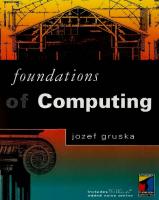
Figure 1.1 H-layout of complete binary trees Example 1.1.1 (H -layout of binary trees) A layout ofa graph G into a two-dimensional grid is a mapping of different nodes of G into different nodes of the grid and edges ( u, v) of G into nonoverlapping paths, along the grid lines, between the images of nodes u and v in the grid. The so-called H-layout Hr2n of a complete binary tree T2n of depth 2n, n 2: 0 (see Figure 1.1a for T2n and its subtrees T2n_2 ), is described recursively in Figure 1.1c. A more detailed treatment of such layouts will be found in Section 10.6. Here it is of importance only that for length L(n) of the side of the layout Hr2" we get the recurrence
L( n) =
{
2 , 2L(n-1)+2,
if n
1; ifn>1. =
As we shall see later, L( n) = 2 n+ 1 - 2. A complete binary tree of depth 2n has 22n+ 1 1 nodes. The total area A(m) of the H-layout of a complete binary tree with m nodes is therefore proportional to the number of nodes of the tree.1 Observe that in the 'natural layout of the binary tree', shown in Figure l.ld, the area of the smallest rectangle that contains the layout is proportional to m!ogm. To express this concisely, we will use the notation A (m) = e ( m ) in the first case and A ( m ) = e ( m lg m ) in the second case. The notationfn ( ) = e(g(n)) -which means that 'f(n) grows proportionally to g(n) 2 -is discussed in detail and formally in Section 1.5. -
'
1 The task of designing layouts of various graphs on a two-dimensional grid, with as small an area as possible,
is of i m portance for VLSI designs. For more on layouts see Section 10.6. 20r, more exactly, that there are constants c .c2 > 0 such that c1\g(n)\ manyn.
1
l. =
(1 .1)
entails fewer ring moves. It is a simple task to show that such an algorithm does not exist. Denote by
In
spite of the simplicity of the algorithm, i t i s natural t o ask whether there exists a faster one that
Tmin (n)
the minimal number of moves needed to perform the task. Clearly,
to
C, then the largest one to
Tmin (n) ? 2Tmin (n
-1) + 1,
B, we have first to move the top n - 1 of them B, and finally the remaining ones to B. This implies that our solution is
because in order to remove all rings from rod A to rod the best possible. Algorithm
1.1.3
is very simple. However, it is not so easy to perform it 'by hand', because of the
need to keep track of many levels of recursion. The second, 'iterative' algorithm presented below is from this point of view much simpler. (Try to apply both algorithms for
Algorithm 1.1.4 (Towers of Hanoi
-
an
n
=
4.)
iterative algorithm)
Do the following alternating steps, starting with step
1, until all the rings are properly transferred:
E�PLES
1. Move the smallest top ring in clockwise order and in
II
5
(A -> B -> C -> A) if the number of rings is odd,
anti-clockwise order if the number of rings is even.
2. Make the only possible move that does not involve the smallest top ring.
In spite of the simplicity of Algorithm 1 . 1 .4, it is far from obvious that it is correct. It is also far from obvious how to determine the number of ring moves involved until one shows, which can be done by induction, that both algorithms perform exactly the same sequences of moves. Now consider the following modification of the Towers of Hanoi problem. The goal is the same, but it is not allowed to move rings from A onto B or from B onto A. It is easy to show that in this case too there is a simple recursive algorithm for solving the problem; for its number T' ( n) of ring moves we have T' (1) = 2 and T' (n) = 3T' (n - 1) + 2, for n > 1 . (1.2)
There is a modem myth which tells how Brahma, after creating the world, designed 3 rods made of diamond with 64 golden rings on one of them in a Tibetan monastery. He ordered the monks to transfer the rings following the rules described above. According to the myth, the world would come to an end when the monks finished their task.3
Exercise 1.1.5 Use both algorithms for the Towers of Hanoi problem to solve the cases (a) n = 3; (b) n = 5; (c) * n = 6. Exercise 1.1.6 •(Parallel version of the Towers of Hanoi problem) Assume that in each step more than one ring can be moved, but with the following restriction: in each step from each rod at most one ring is removed, and to each rod at most one ring is added. Determine the recurrence for the minimal number Tp (n) of parallel moves needed to solve the parallel version of the Towers of Hanoi problem. (Hint: determine Tp ( 1 ) , Tp (2) and Tp (3), and express Tp (n) using Tp (n - 2) .)
The two previous examples are not singular. Complexity analysis leads to recurrences whenever algorithms or systems are designed using one of the most powerful design methods -
divide-and-conquer.
c i , where c, i are integers, using_ the following recursive method, where b1 , b2 and d are constants (see Figure 1.3):
Example 1.1.7 We can often easily and efficiently solve an algorithmic problem P of size n
=
1. Decompose P, in time b 1 n, into su bproblems of the same type and size � 2 . Solve all subproblems recursively, using the same method.
3. Compose, in time b2n, the solution of P from solutions of all its a subproblems.
For the time complexity T( n) of the resulting algorithm we have the recurrence: T(n) =
{ :T
( !! ) + b1 n + b2 n ' c
=
if n 1 ; if n > l .
(1.3)
3Such a prop hecy is not unreasonable. Since T ( n) = - 1 , as will soon be seen, it would take more than 500,000 years to finish the task if the monks moved ring per second.
one
zn
6 • FUNDAMENTALS
a
Figure 1.3
subproblems
Divide-and-conquer method
As an illustration, we present the well-known recursive algorithm for sorting a sequence of n = 2k numbers. Algorithm
1.1.8
(MERGESORT)
1. Divide the sequence in the middle, into two sub sequences -
.
2. Sort recursively both sub-sequences. 3. Merge both already sorted subsequences. If arrays are used to represent sequences, steps (1) and (3) can be performed in a time proportional to n. Remark 1.1.9 Note that we have derived the recurrence (1 .3) without knowing the nature of the problem P or the computational model to be used. The only information we have used is that both decomposition and composition can be performed in a time proportional to the size of the problem.
Exercise 1.1.10 Suppose that n circles are drawn in a plane in such a way that no three circles meet in a point and each pair of circles intersects in exactly two points. Determine the recurrence for the number of distinct regions of the plane created by such n circles.
An analysis of the computational complexity of algorithms often depends quite significantly on the underlying model of computation. Exact analysis is often impossible, either because of the complexity of the algorithm or because of the computational model (device ) that is used. Fortunately exact analysis is not only unnecessary most of the time, it is often superfluous.So-called asymptotic estimations not only provide more insights, they are also to a large degree independent of the particular computing model/ device used. ,
EXAMPLES
•
7
Example 1.1.11 (Matrix multiplication) Multiplication of two matrices A = {a;;}7,;= 1 ' B = {b;; } i,;= 1 of ' degree n, with the resulting matrix C = AB = { c;; }?,;= 1 , using the well-known relat ion C ;;
n
=
2:::aik bkj ,
(1 .4)
k= 1
req u ires T(n) = 2n3 - n2 arithmetical operations to perform. It is again simpler and for the most part sufficiently informative, to say that T(n) = 8 (n3 ) than to write exactly T(n) = 2 n3 - n2 • If a program for computing c;; using the formula (4.3.3) is written in a natural way in a high-level programming language and is implemented on a normal sequential computer, then exact analysis of the number of computer instructions, or the time T(n) needed is almost impossible, because it depends on the available compiler, operating system, computer and so on. Nevertheless, the basic claim T(n) = 8 (n3 ) remains valid provided we assume that each arithmetical operation takes one unit of time.
Remark 1.1.12 If, on the other hand, parallel computations are allowed, quite different results concerning the number of steps needed to multiply two matrices are obtained. Using n3 processors, all multiplications in equation (4.3.3) can be performed in one parallel step. Since any sum of n numbers x1 + . . . + Xn can be computed with � processors using the recursive doubling technique4 in pog2 n l steps, in order to compute all c;; in (4.3.3) by the above method, we need 8( n3 ) processors and e (log n) parallel steps. Example 1.1.13 (Exponentiation) Let bk _1 . . . b0 be the binary representation of an integer n with b0 as the least significant bit and bk- 1 = 1. Exponentiation e = a" can be performed in k = flog2 (n + 1 ) 1 steps using the following so-called repeated squaring method based on the equalities
e=a Algorithm 1.1.14 (Exponentiation)
k- 1
k- 1
i= O
i= O
L = b 2 = II ab;2' = II (a2' ) b' . k-1 . ' ; o ;
begin e +- 1 ; p +- a; for i +- 0 to k 1 do if b; = 1 then e +- e · p; -
p +- p · p
od end
Exercise 1.1.15 Determine exactly the number of multiplications which Algorithm 1 . 1 . 1 4 performs.
Remark 1.1.16 The term 'recurrence' is sometimes used to denote only the equation in which the inductive definition is made. This terminology is often used explicitly in cases where the specific value of the initial conditions is not important. 4 For example, to get x1 + . +xs, we compute in the first step z1 Xt + x2 , z 2 the second step zs z1 + z2 , z6 = Z3 + z4 ; and in the last step Z7 = zs + Z6· . .
in
=
=
=
x3 + x4 , z3
=
xs + x6 , z4 = X7 + xs;
8
•
1 .2
FUNDAMENTALS
Solution of Recurrences - Basic Methods
Several basic methods for solving recurrences are presented in this chapter. It is not always easy to decide which one to try first. However, it is good practice to start by computing some of the values of the unknown function for several small arguments. It often helps
1. to guess the solution; 2. to verify a solution-to-be. Example 1.2.1 For small values of n, the unknown functions T(n) and T' (n) from the recurrences (1 . 1) and (1 .2) have the following values:
n T(n)
1 1
2 3
3 7
5 31
6 63
7 127
8
9
15
255
511
10 1,023
T' (n)
2
8
26
80
242
728
2,186
6,560
19,682
59,049
4
From this table we can easily guess that T(n) = 2" - 1 and T' (n) = 3" - 1 . Such guesses have then to be verified, for example, by induction, as we shall do later for T(n) and T' (n) .
Example 1.2.2 The recurrence
if n = 0; if n = 1 ; if n > 1 ; where a , (3 > 0, looks quite complicated. However, i t is easy to determine that Q2 = (3 , Q3 = a , Q4 = (3. Hence
Qn = 1 .2.1
{
(3,
a,
if n = 3kfor some k; otherwise.
Substitution Method
Once we have guessed the solution of a recurrence, induction is often a good way of verifying the correctness of the guess.
Example 1.2.3 (Towers of Hanoi problem) We show by induction that our guess T(n)
=
2" - 1 is correct.
Since T(1) = 2 1 - 1 = 1, the initial case n = 1 is verified. From the inductive assumption T(n) the recurrence (1 . 1), we get, for n > 1,
1
T(n + 1 ) = 2T(n) + = 2(2" - 1 ) + 1
=
=
2" - 1 and
2"+ 1 - 1 .
This completes the induction step. Similarly, we can show that T' ( n) = 3" - 1 is the correct solution of the modified Towers of Hanoi problem, and L(n) = 2" + 1 - 2 is the length of the side of the H-layout in Example 1.1.1. The inductive step ·in the last case is L(n + 1 ) 2L(n) + 2 = 2(2" + 1 - 2) + 2 = 2"+ 2 - 2. =
SOLUTION OF RECURRENCES - BASIC METHODS • 9
1 .2.2
Iteration Method
Using an iteration (unrolling) of a recurrence, we can often reduce the recurrence to a summation, which may be easier to compute or estimate.
Example 1.2.4 For the recurrence (1.2) of the modified Towers of Hanoi problem we get by an unrolling
3T'(n - 1 ) + 2 = 3(3T' (n - 2) + 2) + 2 = 9T' (n - 2) + 6 + 2 9(3T'(n - 3) + 2) + 6 + 2 = 33 T' (n - 3) + 2 x 32 + 2 x 3 + 2
T'(n)
n-1
n-1
i= O
i= O
'"' 3 i X 2 = 2 '"' 3i = 2 3" - 1 L....t L....t 3-1 Example 1.2.5 For the recurrence T(1) = g(1) and T(n)
=
=
3" - 1 .
T(n - 1 ) + g(n),for n > 1 , the unrolling yields
n
T(n) =
L g(i) . i= 1
Example 1.2.6 By an unrolling of the recurrence
T(n) =
{ !T
if n = 1 ; ( � ) + bn, if n = ci > 1 ;
obtained by a n analysis of divide-and-conquer algorithms, we get T(n)
G) + bn = a (ar (�) + b �) + bn = a2 T (�) + bn � + bn a2 (aT ( �) + b � ) + bn � + bn = a3 T (�) + bn � + bn � + bn aT
Therefore,
""
•
Case 1, a < c:
T(n) = e (n), because the sum L
•
Case 2, a = c:
T(n) = e (n log n).
•
Case 3, a > c:
T(n)
i= O
=
8 (n1ogc•) .
Indeed, in Case 3 we get T(n)
. (�) 1Converges.
I0
II
FUNDAMENTALS
using the identity a log, n
=
n log,a .
Observe that the time complexity of a divide-and-conquer algorithm depends only on the ratio � , and neither on the problem being solved nor the computing model (device) being used, provided that the decomposition and composition require only linear time.
Exercise
1.2.7
Solve the recurrences obtained by doing Exercises
1.1.6
and 1 . 1 . 1 0.
Exercise 1.2.8 Solve the following recurrence using the iteration method:
Exercise
1.2.9
Determine gn , n a power of 2, defined by the recurrence g1
=
3 and gn = (2 ! + 1 )g � for n 2 2.
Exercise 1.2.10 Express T(n) in terms of the function g for the recurrence T(l) = a, T(n) = 2P T ( n / 2) + nPg(n), where p is an integer, n 2k, k > 0 and a is a constant. =
1 .2.3
Reduction to Algebraic Equations
A large class of recurrences, the homogeneous linear recurrences, can be solved by a reduction to algebraic equations. Before presenting the general method, we will demonstrate its basic idea on an example.
Example 1.2.11 (Fibonacci numbers) Leonardo Fibonacci5 introduced in defined by the recurrence
Fo = 0, F1 = 1 Fn Fn -1 + Fn-2 , =
if n > 1
1 202 a
sequence of numbers
(the initial conditions); (the inductive equation) .
(1 .5) (1 .6)
Fibonacci numbers form one of the most interesting sequences of natural numbers:
0 , 1 , 1 , 2, 3, 5, 8, 13 , 21 , 34, 55 , 89, 144, 233, 377 , 610, . . . Exercise 1.2.12 Explore the beauty of Fibonacci numbers: (a) find all n such that Fn = n and all n such that Fn n 2 ; (b) determine L �= 0 F;; (c) show that Fn+ 1Fn - 1 - F� = ( - 1 ) n for all n; (d) show that F2n+ 1 = F� + F�+ 1 for all n; (e) compute F16 , . . . , F49 (F50 = 12, 586, 269, 025 ) . =
5
Leonardo o f Pisa (1170-1250), known also a s Fibonacci, was perhaps the most influential mathematician of medieval Christian world. Educated in Africa, by a Muslim teacher, he was famous for his possession of the mathematical knowledge of both his own and the preceding generations. In his celebrated and influential classic Liber Abachi (which appeared in print only in the nineteenth century) he introduced to the Latin world the Arabic positional system and Hindu methods of calculation with fractions, square roots, cube roots, etc. The following problem from the Liber Abachi led to Fibonacci numbers: How many pairs afrabbits will be produced in a year, beginning the
with a single pair, if in every month each pair bears a new pair which becomes productive from the second month on.
SOLUTION OF RECURRENCES - BASIC METHODS
i
1,
and therefore
either r = 0, which is an uninteresting case, or r2 = r + 1. The
last equation has two roots:
1 + VS
1 - vs r2 = 2- .
Tt = -- , 2
Unfortunately, neither of the functions r'i , r� satisfies the initial conditions in (1.5). We are therefore not ready y et. Fortunately, however, each linear combination .\r'i + w2 satisfies the inductive equation
(1.6). Therefore, if .\ , J.L are chosen in such a way that the initial conditions (1.5) are also met, that is, if (1 .7)
then Fn
= .\r'i + w� is the solution of recurrences (1.5) and (1 .6). From (1 .7) we get .\ =
1
- J.L = vs ,
and thus
Since
(
)
" lim 1 -2.;s = 0, we also get a simpler, approximate expression for Fn of the form
n �oc
Fn
�
_2__ VS
( )
1 + vs " 2
'
for
n --.
oo .
0
The method used in the previous example will now be generalized. Let us consider
homogeneous linear recurrence: that is, a recurrence where the value of the unknown is expressed as a linear combination of a fixed number of its values for smaller arguments: Un = a1 Un- 1 + a2 Un- 2 + · · · + a kUn-k Ui bi , =
where a1 , . . . , ak and b0 , . . . , bk - l
if n if
2 k,
0 :S i < k
(the inductive equation)
(the initial conditions )
a
function
(1 .8) (1 .9)
are constants, and let
rk - La;rk-i i= 1 k
P(r)
=
(1.10)
be the characteristic polynomial of the inductive equation (1.8) and P(r) = 0 its characteristic equation. The roots of the polynomial (1.10) are called characteristic roots of the inductive equation (1 .8). The following theorem say s that we can alway s find a solution of a homogeneous linear recurrence when the roots of its characteristic polynomial are known.
12
•
FUNDAMENTALS
Theorem 1.2.13 (1) If the characteristic equation P(r) = 0 has k different roots r1 , . . . rk , then the recurrence (1 .8) with the initial conditions (1 . 9) has the solution
k
U n = L Ajrj,
(1.11)
j= 1
where >..i are solutions of the system of linear equations k
"L v J ,
b; =
j= 1
o � i < k.
(1.12)
(2) If the characteristic equation P(r) 0 has p different roots, r1 , . . . , rp, p < k, and the root ri, 1 � j � p, 1 has the multiplicity mi ;::: 1, then rj , nrj , n2rj , . . . , nmi - rj, are also solutions of the inductive equation (1 .8), and there is a solution of(1.8) satisfying the initial conditions (1.9) of theform Un "Ej=1 Pi (n)rj, where each Pi ( n) is a polynomial of degree mi - 1, the coefficient of which can be obtained as the unique solution of the system of linear equations b; = "Ej= 1 Pj (i)rj, 1 � i � k. =
=
Proof: (1) Since the inductive equation (1 .8) is satisfied by Un = rj for 1 � j � k, it is satisfied also by an
:
arbitrary linear combination "E = 1 air'/ . To prove the first part of the theorem, it is therefore sufficient to show that the system of linear equations (1.12) has a unique solution. This is the case when the determinant of the matrix of the system does not equal zero. But this is a well-known result from linear algebra, because the corresponding (Vandermond) matrix and determinant have the form
1
det
�- 1 1
1
1 r2
rk
�-1 2
�- 1 k
r1
=
IT (r; - ri) # 0. j> i
(2) A detailed proof of the second part of the theorem is quite technical; we present here only its basic idea. We have first to show that if ri is a root of the equation P(r) = 0 of multiplicity mi > 1, then all . 1 . . func tions Un rin , Un = nrin , Un = n2 rin , . . . , Un nm1· - rin satisfy the .md ucti"ve equation (1 . 8) . "'10 prove this, we can use the well-known fact from calculus, that if ri is a root of multiplicity mi > 1 of the equation P(r) 0, then ri is also a root of the equations (r) is the jth ( r ) 0, 1 � j < mi, where derivative of P(r) . Let us consider the polynomial =
=
pU>
=
Q(r) = r · (r"- k P(r) )
Since P(rj)
'
p (i )
=
r [(n - k)rn - k -l P(r) + r" -k P' (r) ] .
= P' (rj) = 0, we have Q(rj) = 0 . However, Q(r)
=
=
=
·
r[r" - a1 r"-1 - - ak r" -k ] ' nr" - a1 (n - 1)r"- 1 - · · · - ak _ 1 (n - k + 1 ) rn -k+ 1 - ak (n - k)r"- k , · · ·
and since Q(rj ) = 0, we have that Un nrj is the solution of the inductive equation (1 .8). In a similar way we can show by induction that all Un = n'rj, 1 < s < mi , are solutions of (1 .8) by considering the following sequence of polynomials: Q1 (r) = Q(r), Q2 (r) = rQ; (r) , . . . , Q, (r) = =
r0,_ 1 (r) .
It then remains to show that the matrix of the system of linear equations b; is nonsingular. This is a (nontrivial) exercise in linear algebra.
=
"Ef= 1 Pj (i) rj , 1 � i � k, D
SOLUTION OF RECURRENCES - BASIC METHODS
•
13
Example 1.2.14 The recurrence
3Un-1 - 2Un- 2 , n > 2; 1, 0, U1
Un Uo
has the characteristic equation r2 3r - 2 with two roots: r1 2, r2 1. Hence Un = >.12" + >.2, where >.1 = 1 and >.2 - 1 are solutions of the system of equations 0 >. 1 2° + >.2 1 ° and 1 = >.121 + >.21 1 . =
=
=
=
=
Example 1.2.15 The recurrence
Sun-1 - 8un -2 + 4un -3, n :::: 3, 0, u1 = - 1 , u2 2,
Un u0
=
has the characteristic equation r3 = 5r2 - 8r + 4, which has one simple root, r1 1, and one root of multiplicity 2, r2 = 2. The recurrence therefore has the solution Un a + (b + en )2", where a, b, c satisfy the equations
=
-1
0 = a + (b + c - 0)2° ,
=
=
1 a + (b + c - 1)2 ,
2 = a + (b + c · 2)22 .
1.2.16 (a) The recurrence u0 3, u1 5 and Un = Un-1 - Un _2 , fur n > 2, has two roots, x1 = l+�v'3 1�0 , and the solution Un ( � - � ivf3)x;' + ( � + � i vf3)x�. (Verify that all Un are integers!) and x2 (b) For the recurrence u0 = 0, u 1 1 and U n = 2un_1 - 2un_ 2 , fur n 2: 2, the characteristic equation has two roots, x1 = ( 1 + i) and x2 = ( 1 - i), and we get
Example
=
=
=
=
=
�
Un = i ( ( 1 - i)" - (1 + i)")
=
2 � sin(
:),
n
using a well-known identity from calculus.
Exercise 1.2.17 Solve the recurrences (a) u0 = 6, u 1 = 8, Un = 4u n_ 1 - 4un_ 2 , n 2: 2; (b) u0 Un = Sun-1 - 6un- 2 ' n :::: 2; (c) Uo = 4, u1 = 10, Un 6un-1 - 8Un- 2 ' n :::: 2.
=
1,
u1 = 0,
=
Exercise 1.2.18 Solve the recurrences (a) uo = 0, u1 = 1, u2 U1 = -4, U2 8, Un 2un-1 + 5Un-2 - 6Un-3' n 2: 3; (c) Uo =
6Un- 3 ' n 2: 3.
1, Un = 2un-2 + Un-3 , n 2: 3; (b) Uo = 7, 1, U1 = 2, U2 3, Un = 6Un -1 - 1 1Un-2 +
=
=
=
=
Exercise 1.2.19 • Using some substitutions of variables, transform the following recurrences to the cases dealt with in this section, and in this way solve the recurrences (a) u1 = 1, Un Un_1 - UnUn_1, n :::=: 2; (b) U1 0, Un n(u n /2 ) 2 , n is a power of2; (c) Uo 1, U1 = 2, Un = Jun-1 Un - 2, n 2: 2. =
=
=
=
Finally, we present an interesting open problem due to Lothar Collatz (1930), a class of recurrences that look linear, but whose solution is not known. For any positive integer i we define the so-called (3x + 1 ) -recurrence by (a Collatz process) Ubi) = i , and for n > 0,
u n( i+J 1 =
{
UJ �
3u �i ) + 1, 2 ,
if u �i ) is even; if u �i l is odd.
B
14
FUNDAMENTALS
3
2
3
-3
l XJ
. I Xl
-3
Figure 1.4 Ceiling and floor functions It has been verified that for any i < 240 there exists an integer n; su ch that u�:J = 1 (and therefore 4, u �:� 2 2, u�:J+ 3 1 , . . . ). However, it has been an open problem since the early 1950s - the so-called Collatz problem - whether this is true for all i.
u �:J+ l
=
=
=
i Exercise 1.2.20 Denote by a(n) the smallest i such that u � ) (b)* a(250 - 1 ), a(250 + 1 ) , a(2500 - 1 ), a( 2500 + 1 ) .
1.3
< n. Determine (a) a(26), a(27), IT(28);
Special Functions
There are several simple functions that are often used in the design and analysis of computing systems. In this section we deal with some of them: ceiling and floor functions for real-to-integer conversions, logarithms and binomial functions. Despite their apparent simplicity, these functions have various interesting properties and also, as discussed later, surprising computational power in the case of ceiling and floor functions.
1 .3.1
Ceiling and Floor Functions
Integers play an important role in computing and communications. The same is true of two basic reals-to-integers conversion functions.
Floor: Ceiling:
lxJ - the largest integer � x Ixl - the smallest integer :::: x
For example, l3 . 14j = l3 . 14l =
3 4
l3 . 75J , = l3 . 75l , =
l -3 . 14J = l -3 . 14l =
-4 -3
= =
l-3. 75J ; l-3. 75l
•
SPECIAL FUNCTIONS
IS
The following basic properties of the floor and ceiling functions are easy to verify: lx + n J = lx J + n and Ix + n 1
lx J
Ix 1
= x O ;;r1 Zn
Table 1 . 2 Generating functions for some sequences and their closed forms
Exercise 1.4.4
Find a closed form of the generating function for the seq uences
0 �,0, �,0, �' . . . ) .
( a ) an = 3" + 5" + n, n � 1; (b) (0 , 2 , ,
such that [z"]F(z) = Li= O ( 7) ( n � i),for n � 1 . 2 2 Use generating functions to show that L�= 0 (7) = e:)
Exercise 1.4. 5 • Find a generating function F(z) Exercise 1.4.6
1 .4.2
0
Solution of Recurrences
The following general method can often be useful in finding a closed form for elements of a sequence (gn) defined through a recurrence Step
1
Form a single equation in which gn is expressed in terms of other elements of the sequence. It is important that this equation holds for any n; also for those n for which g. is defined by the initial values, and also for n < 0 (assuming gn 0). =
Step 2 Multiply both sides of the resulting equation by z" , and sum over all n. This gives on the left-hand side G(z) = Egn z" - the generating function for (g. ). Arrange the right-hand side in such a way that an expression in terms of G(z) is obtained. Step
3
Solve the equation to get a closed form for G(z) .
SOLUTION OF RECURRENCES - GENERATING FUNCTION METHOD
•
23
Step 4 Expand G(z) into a power series. The coefficient of z" is a closed form for gn .
Examples In the following three examples we show how to perform the first three steps of the above method.
Later we present a method for performing Step 4 - usually the most difficult one. This will then be applied to finish the examples. In the examples, and also in the rest of the book, we use the following mapping of the truth values of predicates P( n ) onto integers: [P( n
)]
=
{
1,
0,
if P(n) is true; if P(n) is false .
Example 1.4.7 Let us apply the above method to the recurrences (1.5) and (1 . 6) for the initial conditions f0 = 0, f1 1 and the inductive equation
Fibonacci numbers with
=
fn fn-1 +fn-2> n > 1 . =
Step 1 The single equation capturing both the inductive step and the initial conditions has the form
fn = fn-1 +fn-2 + [n = 1] . and this is important - that the equation is valid also for n S: 1, because fn Step 2 Multiplication by z" and a summation produce
(Observe -
n
n
n
zF(z) + rF(z) + z.
=
Step 3 From the previous equation we get
F (z ) = Example 1.4.8
z z - z2 . 1
Solve the recurrence 1, 2,
2gn- 1 + 3gn-2 + ( - 1)" , Step
1
A single equation for gn has the form
ifn = 0 ; if n 1 ; ifn > l . =
=
0 for n < 0.)
•
24
FUNDAMENTALS n
I�
u.
(a)
n
l
(b)
n
II
v •. ,
n
v•. ,
+
+
u n- 2
n
v.
Figure 1.5
n
u n-
n
+
1
vn 2
Recurrences for tiling by dominoes
Step 2 Multiplication by z"
and summation give
L ( 2gn-l + 3gn-2 + ( - 1 )"[n � 0] + [n = 1 ]) z" n
L 2gn-lz" + 3 L gn- 2 Z" + L(-1)"z" + L z" n;::O n n= l n 1 + z. 2zG (z ) + 3z2 G(z) I
1 + -
+z
Step 3 Solving the last equation for G(z), we get
G (z)
=
z2 +z + 1 (1 + z) 2 (1 - 3z) ·
As illustrated by the following example, the generating function method can also be used to solve recurrences with two unknown functions. In addition, it shows that such recurrences can arise in a natural way, even in a case where the task is to determine only one unknown function.
Example 1.4.9 (Domino problem)
identical dominoes of size 1 x 2.
Determine the number u. of ways of covering a 3 x n rectangle with
Un = 0 for n 1 3 and u 2 3. To deal with the general case, let us introduce a new variable, v., to denote the number of ways we can cover a 3 x n with-a-comer-rectangle (see Figure 1 .5b) with
Clearly
=
=
,
such dominoes . For the case get the recurrences
n
=
0 we have exactly one possibility: to use no domino. We therefore
U 1 , u1 = 0; Un 2Vn- 1 + Un-2 ; o =
Vo =
=
=
Let u s now perform Steps 1 -3 o f the above method.
Step 1 U n
=
2Vn -·l
+ Un - 2 + [n = OJ ,
Vn
0,
V1
=
1;
Vn Un-l + Vn- 2 ,
=
Un-1 + Vn - 2 ·
n
� 2.
SOLUTION OF RECU RRENCES - GENERATING FUNCTION METHOD
Step 2 U(z) = 2zV(z) + z2 U(z) + 1 , Step
3
• 25
V(z) = zU(z) + z2 V(z) .
The solution of this system of two equations with two unknown functions has the form U(z)
=
z
1
V(z)
1- 2 - 4z2 + z4 '
=
z 1 - 4z2 + z4 .
A general method of pedorming step 4
In the last three examples, the task in Step 4 is to determine the coefficients [z"]R(z) of a rational function R(z) P(z) I Q(z) . This can be done using the following general method. If the degree of the polynomial P(z) is greater than or equal to the degree of Q(z ) , then by dividing P(z) by Q(z) we can express R(z) in the form T(z) + S(z), where T(z) is a polynomial and S(z) P1 (z) I Q ( z) is a rational function with the degree of P1 (z) smaller than that of Q (z) Since [z"]R(z) [z"] T(z) + [z"]S(z), the task has been reduced to that of finding [z"]S(z). From the sixth row of Table 1 .2 we find that =
=
.
=
a
{ 1 - pz) m + l
=
(
)
'""" m + n apn zn , � n n 2:0
and therefore we can easily find the coefficient [z ] S (z ) in the case where S(z) has the form "
(1 .22)
for some constants a; , p; and m; , 1 .,; i .,; m. This implies that in order to develop a methodology for performing Step 4 of the above method, it is sufficient to show that S(z) can always be transformed into either the above form or a similar one. m In order to transform Q(z) = qo + q1z + · qmz into theform Q(z) = qo (l - p1z) (1 - P2Z) . . . (1 - PmZ), we need to determine the roots l , . . , .l.. of Q(z) . Once these roots have been found, one of the following theorems can be used to perform Step 4. · ·
PI
.
Pm
� ' where Q(z) = q0 (1 - p1z) . . . ( 1 - Pmz), the numbers p1 , . . . , pm are distinct, and the degree of P1 (z) is smaller than that ofQ(z), then
Theorem 1.4.10 IfS(z) =
where
Proof: It is a fact well known from calculus that if all p;
where
a1 ,
.
.
.
, a1 are constants, and thus
are different, there exists a decomposition
26
•
FUNDAMENTALS
Therefore, for i = 1 ,
.
.
.
,
1
,
ai = lim/ ( 1 - PiZ)R(z) , z�l p,
and using !'Hospital's rule we obtain
0
where Q' is the derivative of the polynomial Q.
The second theorem concerns the case of multiple roots of the denominator. For the proof, which is more technical, see the bibliographical references.
Theorem 1.4.11 Let R(z) = ���\ , where Q(z) of P (z) is smaller than that of Q(z); then
=
q0 ( 1 - p1z) d1
.
.
. ( 1 - p1z) d1 ,
Pi
are distinct, and the degree
where each f; ( n) is a polynomial of degree di 1, the ma in coefficient of which is -
where Q(dj) is the i-th derivative of Q. To apply Theorems 1 .4.10 and 1 .4.11 to a rational function &ffi with Q(z) = q0 + q 1 z + · · · + qmzm , we must express Q(z) in the form Q(z) q0 ( 1 - p1 z) d 1 ( 1 - Pm Z)dm . The numbers -J;; are clearly roots of Q(z) . Applying the transformation y = t and then replacing y by z, we get that Pi are roots of the 'reflected' polynomial � ( z ) = q m + q m- 1 Z + · · · + qozm , =
•
•
•
and this polynomial is sometimes easier to handle.
Examples - continuation Let us now apply Theorems 1 .4.10 and 1 .4.11 to finish Examples 1 .4.7, 1 .4.8 and 1 .4.9. In Example 1 .4.7 it remains to determine [z " ] 1 z2 . -
The reflected polynomial z2
-
z 1 has two roots:
Theorem 1 .4.10 therefore yields
-
:
-
SOLUTION OF RECURRENCES - GENERATING FUNCTION METHOD
To finish Example
27
1.4.8 we have to determine g
..
n
1 + z + z2
[z ] (1 - 3z) (1 + z) 2
=
The denominator already has the required form. Since one root has multiplicity Theorem
•
1 .4.11. Calculations yield
�
g.. = ( n + c) ( -1)" + The cons tant c = � can be determined remains to determine
[z" ] U (z)
=
!� 3".
using the equation 1 = g0
[z"] 1 _\�2�z4
=
2,
we need to use
c + � - Finally, in Example 1 .4.9, it (1 .23)
and
In order to apply our method directly, we would need to find the roots of a polynomial of degree
4. But this, and also the whole task, can be simplified by realizing that all powers in (1 .23) are even. Indeed, if we define
1
W ( z) = -o4z_ . +_z-=-2 ' 1- ....,. then
+
Therefore
[z2n l]U(z) [z2"] V(z)
0, 0,
where
Wn = [z"] 1 which is easier to determine.
� - z2 '
Exercise 1.4.12 Use the generating function method to solve the recurrences in Exercises 1 .2. 1 7 and 1 .2.18. Exercise 1.4.13 Use the generating function method to solve the recurrences 0, U 1 1 , Un u - n - 1 + Un- 2 + ( -1 ) " , n 2: 2; 0, ifn < 0, go = 1 and g gn -1 + 2gn - 2 + . . . +ngo for n > 0.
..
(a) Uo (b) g
=
=
=
=
..
=
Exercise 1.4.14 Use the generating function method to solve the system of recurrences a0 an = San-1 + 12b,_1, .b,. = 2an -t + 5b,_1, n 2: 1 .
=
1, b0
=
0;
Remark 1.4.15 In all previous methods for solving recurrences i t has been assumed that all components - constants and functions - are fully determined. However, this is not always the case in practice. In general, only some estimations of them are available. In Section 1 .6.2 we show how to deal with such cases. But before doing so, we switch to a detailed treatment of asymptotic estimations.
•
28
1 .5
FUNDAMENTALS
Asymptotics
Asymptotic estimations allow one to produce often surprisingly simple, deep, powerful, useful and technology independent analysis of the performance or size of computing systems. They have contributed much to the rapid development of a deep, practically relevant theory of computing.
In the asymptotic analysis of a function T(n) (from integers to reals) or A (x) (from reals to reals), estimation in limit of T(n) for n ---> oo or A(x) for x ---> a, where a is a real. The
the task is to find an
aim is to determine as good an estimation as possible, or at least good lower and upper bounds for it.
The key underlying problem is how to compare 'in a limit' the growth of two functions. The main approaches to this problem, and the relations between them, will now be discussed. An especially important role is played here by the
0-, !1 -
and 8 -notations and we shall discuss in detail ways of
handling them. Because of the special importance and peculiarities of asymptotic estimations, a discussion of their merits seems appropriate. There is a quite widespread illusion that in science and technology exact solutions, analyses and so on are required and to be aimed for. Estimations are often seen as substitutes, when exactness is not available or achievable. However, this does not apply to the analysis of computing systems . Simple,
good estimations are what are really needed. There are several reasons for this.
Feasibility.
Exact analyses are often not possible, even for apparently simple systems. There are
often too many factors of enormous complexity involved. For example, to make a really detailed time analysis of even a simple program one would need to study complicated compilers, operating systems, computers and, in the case of multi-user systems, the patterns of their interactions.
Usefulness.
An exact analysis could be many pages long and therefore all but incomprehensible.
Moreover, as the results of asymptotic analysis indicate, most of it would be of negligible importance.
In addition, what we really need
are results of analysis of computing systems that are independent
of the particular computer and, in general, of the underlying hardware and software technology. What we require are estimations that are some kind of invariants of computing technologies. Various constant factors that reflect these technologies are not of prime interest. Finally, what is most often needed is not knowledge of the performance of particular systems for particular data, but knowledge about the growth of the performance of systems as a function of the growth of the size of their input data. Again, factors with negligible growth and constant factors are not of prime importance for asymptotic analysis, even though they may be of great importance for applications.
Example 1.5.1 How much time is needed to multiply two n-digit integers (by a person or by a computer) when a classical school algorithm is used ? The exact analysis may be quite complicated. It also depends on many factors: which of many variants of the algorithm is used (see the one in Figure and the computer on which it is
more time is needed to multiply
1 .6), who
executes it, how it is programmed,
k2 times k times larger integers. We can therefore say, simply and in full
run.
However, all these cases have one thing in common:
generality, that the time taken to multiply two integers by a school algorithm is
8 (n2) . Note that this
result holds no matter what kind of positional number system is used to represent integers: binary, ternary, decimal and so on. It is also important to realize that simple, well-understood estimations are
of great importance
even when exact solutions are available. Some examples follow.
Example 1.5.2 In the analysis of algorithms one often encounters so-called harmonic numbers:
ASYMPTOTIC$ • 29
•
•
•
•
•
•
•
•
•
•
•
•
•
•
•
•
•
•
•
•
Figure 1.6 Integer multiplication
Hn
=
1+
� � +···+ �
L i. n
+
=
(1 .24)
i= l
Using definition (1.24) we can determine Hn exactly for any given integer n. This, however, is not always enough. Mostly what we need to know is how big Hn is in general, as a function of n, not for a particular n. Unfortunately, no closed form for Hn is known. Therefore, good approximations are much needed. For example, for n > 1.
In n < H. < In n + 1 ,
This i s often good enough, although sometimes a better approximation i s required. For example,
Example
1.5.3
Hn
=
Thefactorial n!
=
ln n + 0. 5772156649 + 2n
1
1 · 2·
-
1
2
1 n
2
-
+ 8 (n - 4 ) .
. . ·n is another function of importancefor the analysis ofalgorithms.
The fact that we can determine n! exactly is not always good enough for complexity analysis. The following approximation, due to James Stirling (1 692-1 770), .
may be much more useful. For example, this approximation yields lg n!
1 .5.1
=
8 (n log n) .
An Asymp totic Hierarchy
An important formalization of the intuitive idea that one function grows essentially faster than another function is captured by the relation -< defined by
f(n)
-< g(n)
1, lie ? Clearly; lg lg n -< (1Igti -< c lg n, for any c > 0, and therefore, by (1.27), 2 1 g l g n -< 2 � -< 2' 1 g " . Since 2 1 s l s n = lg n and 2d g n = n', we get
lg n -< 2 � -< n' . Exercise 1.5.5 Which of the functions grows faster: (a) n ( l n n ) or (In n)"; (b) (I n n) ! or n1n nln l n n ? In a similar way, we can formalize the intuitive idea that two functions f(n) and
g(n) have the
same rate of growth, as follows:
f(n) "' g(n)
0 :
cjg(n) l
S lf (n) j } .
introduced in 1892 by the German mathematician P. H . B achmann (1837-1920 ). lt Edmund Landau
became more widely known through the work of another German mathematician,
(1877-1938)
and came to be known as Landau notation. However, it was actually D. E. Knuth who
introduced the 0- an d
8-notation and popularized these notations.
8(g(n)), a(g(n) ) and O (g(n)) are sets of functions. However, instead of
f(n)
we u su ally write
f( n )
E
8 (g (n ) ) ,
f(n)
E
a(g(n) ) ,
8 (g(n) ) ,
f( n )
=
a(
g (n ) ) ,
f( n) f(n)
E
O (g(n) ) , O (g ( n ) ) .
There are two reasons for using this notation with the ' equals' sign. The first is tradition. a-notation with the equals sign is well established
in mathematics, especially in number theory. Moreover, we Hn = 8 (lg n) as 'Hn is a big theta of lg n'. The second reason
often read ' = ' as 'is'. For example, we read
is that in asymptotic calculations, as will be illustrated later, we often need to use this notation in the middle of an expression. Our intuition is better satisfied if we interpret the equals sign as signifying
equality rather than inclusion, as discussed later.
32 • FUNDAMENTALS clg(n)l
lf(n)l
/
f(n)
=
f( n ) = O (g ( n) )
e (g ( n ) )
f( n )
=
!1 (g( n ) )
Figure 1.7 Asymptotic relation between functions Relations between functions f(n) and g(n) such thatf(n) = 8 (g(n ) ) , orf(n) = !1 (g( n ) ) or f(n) = O(g( n)) are illustrated in Figure 1 .7. Transitivity is one of the basic properties of 0-, 8- and !1-notation . For example,
f (n )
=
O (g ( n ) ) and g ( n )
=
CJ( h ( n ) )
=*
f (n )
=
CJ (h( n ) ) .
0-, 8- and n-notations are also used with various restrictions on the variables. For example, the notation
f (n )
=
for n --> oo
8 (g ( n ) )
(1.32)
means that there are c1 , c2 > 0 and n0 such that c1 lg(n) l s lf(n) I s c2 lg( n ) I for n :::=: no. Note that the notation 8 (/ (n ) ), and also 0- and !1-notations are very often used as in (1 .32), without writing n --> oo explicitly.
Example 1.5.6 In order to show that (n + lf or, after dividing by n 2 , c1 s 1 +
Example 1.5.7 To show that
For n
>
=
8 (n 2 ) , we look for c1 , c2 > 0 such that
c1 n 2 s l n 2 + 2n + 1 1 s c2n 2 , for n > 0,
� + � s c2 • This inequality is satisfied, for example, with c1
:;i = 8 ( n ) , for n --> 2
oo,
we need constants c1 , c2 > 0 such that
1, this is equivalent to finding c1 , c2 such that c1 n s I n - 1 1 s c2n, or, equivalently,
This inequality is satisfied for n
Example 1.5.8 Since
>
1 with c 1
=
� and c2
=
=
1.
1 and c2
=
4.
ASYMPTOTIC$
we get
2 )* n
=
i� l
Example 1.5.9 To prove that 4n3 =I a(n2 ) for n
•
33
a(n*+ 1 ) . let us assume that there are
4 n3 S c, n2 , fvr n 2: no. This would imply n S c1 I 4 fvr all n 2: n0 - a contradiction. ---> oo,
c1
and n0 such that
The 8-, a- and 0-notations are also used for functions with variables over reals and for convergence to a real. For example, the notation
f(x) means that there are constants
Example 1.5.10 x2
=
=
for x
a (g(x) )
c, r:: > 0 such that lf ( x) I
a(x) for x ---+ 0.
Exercise 1.5.11 Show that (a) lxJ lxl
S c lg (x ) I
=
for 0
8 (x2); (b) (x2 +
---> 0
< l xl ::;
r:: .
1) I (x + 1 ) = e ( x).
Exercise 1.5.12 Give as good as possible an a-estimation fvr the following functions:
(a) (n ! + 3" ) ( n2 + log(n3 + 1 )); (b) ( 2" + n2 ) (n3 + s n ); (c) n2" + n"2 •
The a-notation has its peculiarities, which we shall now discuss in more detail. Expressions of the
type f ( n )
=
a (g (n ) ) , for example,
3 2 2 n - 2n + 3n - 4 1
=
a ( n3 )
,
should be seen as one-way-equalities, and should never be written with the sides reversed. Thus, we should not write a(n3 ) = ! n3 - 2n2 + 3n - 4. This could lead to incorrect conclusions. For example,
3
2
=
2
from n a( n ) and a(n3 ) n one might be inclined to conclude that n a(n3) n . This does not mean that a-notation cannot be used on the left-hand side of an equation. It has only to be dealt with =
=
=
properly and interpreted consistently as a set of functions. One can also write a(g1 ( n ) ) + a(g2 ( n ) ) or a(g1 ( n ) ) · a (g (n) ), and so on, with the usual interpretation of operations on sets. For example,
2
We can therefore write
2n + a(n 2) + a ( n3 )
which actually means that 2n + a(n2)
+ a( n3 ) � a(n3 ) .
=
a ( n3 ) ,
I f th e a-notation i s used in some environment, i t actually represents a set of functions over all
variables that are 'free' in that environment. Let us illustrate this by the use of a-notation within a sum. This often happens in the analysis of algorithms. We show the identity
•
34
FUNDAMENTALS
The expression 2k 2 + O(k) represents, in this context, a set of functions of the form 2k2 +f(k, 11), for which there is a constant c such that f( 11 , k) ::; ck, for 0 ::; k ::; 11. Therefore n
n
n
k� O
k� o
k� O
E 2k2 +f(k, n) ::; 2 E k2 + c �:)
(1 .33) (1 .34)
(1 .35)
In complexity analysis it often happens that estimations depend on more than one parameter. For example, the complexity of a graph algorithm may depend on the number of nodes and also on the number of edges. To deal with such cases, the 0-, e- and n-notations are generalized in a natural way. For example, Oif(m , n ) )
=
{g(m, n) ! 3c, no : lf(m, n) l :S c !g(m , n) l , for all n � no , m � no } .
Notation 0 is sometimes used also to relate functionsf , g : r ---> N, where r is an arbitrary infinite set. = O(g(x) ) then means that there exists a constant c such thatf(x) ::; cg (x) for almost all x E r .
f ( x)
Exercise 1.5.13 S how t hat (a) n• any a > O, b > 1 .
=
O ( nb ) ifO ::; a ::; b; (b)
a" = O (b" ) if l ::; a ::; b; (c) n•
=
O ( b" ) ,for
Exercise 1.5.14 Show that (a) n! is not 0(2"); (b) nn is not O(n!). Exercise 1.5.15 Show that f(n) = O ( nk ) for some k if and only iff(n) ::; knk for some k > 0.
Remark 1.5.16 One of the main uses of 8-, n- and 0-notations i s i n the computational analysis o f algorithms. For example, in the case of the running time T(n) o f a n algorithm the notation T( n ) = E> if(n ) ) means thatf(n) is an asymptotically tight bound; notation T(n) O.lf(n) ) means that f(n) is an asymptotic lower bound; and, finally, notation T ( n) Olf ( n ) ) means that f ( n) is an asymptotic upper bound. =
=
1 .5.3
Relations between Asymptotic Notations
The following relations between 0-, e- and n-notations follow directly from the basic definition:
f( n) f ( n)
= =
O(g ( n) ) E> (g(n ) )
O, m \ k and n \ k} .
(1 .55)
To compute gcd(m, n), 0 � m < n, we can use the following, more than 2,300-year-old algorithm, a recurrence.
Algorithm 1.7.1 (Euclid's algorithm) For 0 � m < n, gcd(O, n ) gcd(m, n)
=
=
n; gcd (n mod m , m ) ,
for m > 0.
For example, gcd (27 , 36) gcd (9, 27) 9; gcd (214, 352) = gcd ( 138, 214) gcd(0, 9) gcd(76, 138 ) gcd (62, 76 ) gcd ( 1 4 , 62) = gcd (6, 14 ) = gcd (2, 6 ) gcd(0, 3) = 3. Euclid's algorithm can also be used to compute, given m � n, integers n' and m' such that =
=
=
=
=
=
m'm + n'n
=
gcd(m, n ) ,
and this i s one o f its most important applications. Indeed, i f m = 0 , then m ' 0 and n ' = 1 will do. Otherwise, take r = n mod m, and compute recursively r'' , m" such that r"r + m"m gcd(r, m). Since r n - Ln I m J m and gcd(r, m) gcd(m, n), we get =
=
=
=
r" (n - ln I mj m) + m"m = gcd(m, n)
=
(m" - r" Ln I mJ )m + r"n.
If Euclid's algorithm is used, given m, n, to determine gcd(m, n ) and also integers m' and n' such that m'm + n'n = gcd(m, n), we speak of the extended Euclid's algorithm
Example 1.7.2 For m = 57, n
=
237 we have gcd(57, 237) = gcd(9, 57) = gcd ( 3, 9) = 3. Thus 4 · 57 + 9,
237 57
=
6 · 9 + 3,
and therefore 3 = 57 - 6 · 9 = 57 - 6 · (237 - 4 · 57) = 25 · 57 - 6 · 237.
42
•
FUNDAMENTALS
If gcd ( m , n ) = 1, we say that the numbers n and m are relatively prime - notation n _1_ m. The above result therefore implies that if m, n are relatively prime, then we can find, using Euclid's algorithm, an integer denoted by m - 1 mod n, called the multiplicative inverse of m modulo n, such that
m(m - 1 mod n)
=
1 ( mod n)
Exercise 1.7.3 Compute a, b such that ax + by = gcd(x,y) for the following pairs x, y: (a) ( 34 , 5 1 ); (b) (315, 53); (c) (17, 71 ) . Exercise 1.7.4 Compute (a) 17-1 mod 13; (b) 7 - 1 mod 1 9; (c) 3 7 - 1 mod 97.
Analysis of Euclid's algorithm Let us now tum to the complexity analysis of Euclid's algorithm. In spite of the fact that we have presented a variety of methods for complexity analysis, they are far from covering all cases. Complexity analysis of many algorithms requires a specific approach. Euclid's algorithm is one of them. The basic recurrence has the form, for 0 < m ::; n,
gcd ( m , n ) = gcd (n mod m , m ) .
This means that after the first recursive step the new arguments are ( n1 , m ) , with n 1 = n mod m , and after the second step the arguments are ( m 1 , n 1 ) , with m 1 m mod n 1 . Since a mod b < � for any 0 < b < a (see Exercise 49 at the end of the chapter), we have m1 ::; I , n1 ::; � . This means that after two recursion steps of Euclid's algorithm both arguments have at most half their original value. Hence T(n) = O(lg n) for the number of steps of Euclid's algorithm if n is the largest argument. This analysis was made more precise by E. Lucas (1884) and Lame (1884) in what was perhaps the first deep analysis of algorithms. It is easy to see that if Fn is the nth Fibonacci number, then after the first recursive step with arguments (Fn , Fn- 1 ) we get arguments (Fn-l > Fn-2 ) · This implies that for arguments (Fn , Fn- 1 ) Euclid's algorithm performs n - 2 recursive steps. Even deeper relations between Euclid's algorithm and Fibonacci numbers were established. They are summarized in the following theorem. The first part of the theorem is easy to prove, by induction using the fact that if m ::::: Fk + 1 , n mod m ::::: Fk , then n :;::.: m + (n mod m) ::::: Fk + 1 + Fk Fk + 2 · The second part of theorem follows from the first part. =
=
Theorem 1.7.5 (1) If n > m :;::.: 0 and the application of Euclid's algorithm to arguments n , m results in
k
recursive steps, then n ::::: Fk+ 2 , m ::::: Fk+ I · (2) If n > m ::::: 0 ,m < Fk + 1 , then application of Euclid's algorithm to the arguments n , m requires fewer than k recursive steps.
Remark 1.7.6 It is natural to ask whether Euclid's algorithm is the fastest way to compute the greatest common divisor. This problem was open till 1989, and is discussed in more detail in Section 4.2.4.
PRIMES AND CONGRUENCES
1 . 7.2
• 43
Primes
A positive integer p > 1 is called prime if it has just two divisors, composite. The first 25 primes are as follows:
1 and p; otherwise it is called
2, 3,5, 7, 11 , 13, 17, 19, 23, 29, 31, 37, 41 , 43, 47, 53, 59, 61, 67, 71, 73 , 79, 83, 89, 97. Primes play a central role among integers and also in computing. This will be demonstrated especially in the chapter on cryptography. The following, easily demonstrable theorem is the first reason for this. Theorem 1.7.7 (Fundamental theorem of arithmetic) Each integer n has a unique prime decomposition of the form n = n;= I p;i ' where Pi < Pi+ i = 1' . . . ' k - 1, are primes and ei are integers. I'
There exist infinitely many primes. This can easily be deduced from the observation that if we take primes p 1 , . . . , Pk . none of them divides p1 P2 . . . ·pk + 1 . There are even infinitely many primes of special forms. For example, ·
Theorem 1 .7.8
·
There exist infinitely many primes of the form 4k + 3.
Proof: Suppose there exist only finitely many primes p1 , p2 , . . . , p, of the form 4k + 3, that is, pi mod 4 = 3, 1 :S i :S s. Then take N = 4 p1 • p2 . ·p, - 1. Clearly, N mod 4 = 3. Since N > Pi , 1 :S i :S s, N cannot be a prime of the form 4k + 3, and cannot be divided by a prime of such a form. Moreover, since N is odd, N is also not divisible by a number of the type 4k + 2 or 4k. Hence N must be a product of primes of the type 4k + 1. However, this too is impossible. Indeed, ( 4k + 1) ( 41 + 1) = 4(kl + k + I) + 1; for any integers k, I , therefore any product of primes of the form 4k + 1 is again a number of such a form - but N is of the form 4k + 3. In this way we have ruled out all possibilities for N, and therefore our assumption, that the number of primes of the form 4k + 3 is finite, must be wrong. D ·
· .
.
The discovery of as large primes as possible is an old problem. All primes up to 107 had already been computed by 1909. The largest discovered prime at the time this book went to press, due to D. Slowinski and Gage in 1996: using computer Cray T94 is 21 257787 - 1 and has 378,632 digits.6 Another important question is how many primes there are among the first n positive integers; for this number the notation 7r(n) is used. The basic estimation 7r(n) = e c:" ) was guessed already by Gauss7 at the age of 15. Better estimations are
n lnn
is the Euler phi function. ¢>(n) is the number of positive integers smaller than n that are relatively prime to n for example, ¢>(p) p - 1 and ¢> ( pq ) (p - 1) ( q - 1) if p, q are primes.
-
=
Theorem 1.7.9 (Prime number theorem) 8 If
form bk + c we have
gcd b, c (
=
)=
1, then for the number 1rb,c (n) of primes of the
The following table shows how good the estimation 1r(n) = n l ln n is. n
7r(n ) n j ln n 1r(n) I (n I In n)
1, 229 664, 579 455,052, 511 1, 089 621, 118 434, 782, 650 1. 128 1 . 070 1. 046
The largest computed value of 1r(x) is 7r(1018) = 24, 739, 954, 287, 740, 860, by Deliglise and Rivat in 1994. We deal with the problem of how to determine whether a given integer is a prime in Section 5.6.2 and with the problem of finding large primes in Section 8.3.4. The importance of primes in cryptography is due to the fact that we can find large primes efficiently, but are not able to factorize large products of primes efficiently. Moreover, some important computations can be done in polynomial time if argument is prime, but seem to be unfeasible if the argument is an arbitrary integer.
an
Exercise 1.7.10 Show that if n is composite, then so is 2n - 1. Exercise 1.7.11
1 .7.3
.... Show that there exist infinitely many primes
of the type 6k + 5.
Congruence Arithmetic
The modulo operation and the corresponding congruence relation
a = b (mod m) a mod m b mod m (1.57) defined for arbitrary integers a, b and m > 0, play an important role in producing (pseudo-)randomness and in randomized computations and communications. We read 'a = b (mod m)' as 'a is congruent to b modulo m'. From (1.57) we also get that a = b (mod m) if and only if a - b is a multiple of m. =
This congruence defines an equivalence relation on Z, and its equivalence classes are called residue classes modulo n. Zn is used to denote the set of all such residue classes, and Z� its subset, consisting of those classes elements of which are relatively prime to n. 8 The term 'prime number theorem' is also used for the Gauss estimation for n(n) or for the estimation (1 .56).
PRIMES AND CONGRUENCES
•
45
The following properties of congruence can be verified using the definition (1 .57) :
a = b and c d (mod m) => a + c = b + d (mod m) ; a b and c d ( mod m) a - c = b - d ( mod m) ; a = b and c d (mod m) ac bd (mod m ) ; ad = bd (mod m) {=} a = b (mod m) for d ..L m; ad = bd (mod md) a = b (mod m) for d # 0; a = b ( mo d mn) {=} a = b (mod m) and a = b (mod n) if m ..L n.
(1 .58)
=
=
=
=>
=
=>
(1 .59)
(1.60)
=
(1.61) (1 .62)
{=}
(1 .63)
The property (1 .63) can be used to simplify the computation of congruences as follows. If Il�= 1 p;; is the prime decomposition of m, then (1 .64)
Congruences modulo powers of primes are therefore building blocks for all congruences modulo integers. Exercise 1.7.12
Show that ( (a mod n) (b mod n)
Exercise 1.7.13
Show that 2xi mod (2"!1 - x) = xY .
mod
n) = ab mod n for any integers a, b, n.
One of the main uses of the modulo operation in randomization is related to the fact that solving 'nonlinear' congruence equations is in general a computationally intractable task. By contrast, the linear congruence equations
ex = d (mod m) are easy to deal with. Indeed, we have the following theorem. Theorem 1.7.14 A linear congruence ex = d (mod m) has a solution ifand only ifd is a multiple ofgcd(c, m) . In this case, the equation has exactly k = gcd(c, m ) distinct integer solutions m . . x d k 1) m xo dk , xo kd + k ' . , ok + ( - k'
in the interval (0, m ) , where x0 is the unique integer solution of the equation ex + ym be found using Euclid's algorithm.
=
gcd(c, m)
The proof is easy once we realize that the problem in solving the equation equivalent to the one in finding integer solutions to the equation ex + ym d. Another useful fact is that if ex = d (mod m), then c(x + m) = d (mod m).
- which can
ex = d (mod m)
is
=
Example 1.7.15 For the congruence 27x 1 (mod 47) we have g cd( 27 , 47) 1 and 7 · 27 - 4 · 47 1. Hence x = 7 is the unique solution. Example 1.7.16 For the congruence 5 1 x 9 (mod 69) we have gcd(51 , 69) = 3 and -4 · 51 + 3 · 69 = 3. Hence x = -12, 1 1 , 34, or, expressed using only positive integers, =
=
=
X=
11 , 34, 57.
=
II
46
FUNDAMENTALS
Exercise 1.7.17
Solve the linear congruence equations (a) 4x = 5 (mod 9); (b) 2x = 17 (mod 19).
There is an old method for solving special systems of linear congruences. The following result, easy to verify, has been attributed to Sun Tsii of China, around AD 350. Theorem 1.7.18 (Chinese remainder theorem) Let m 1 , , m1 be integers, m; , a1 be integers with 0 < a; < m;. Then the system of congruences •
a1 ,
.
.
•
x = a;
•
•
_i
mi for i
=J. j,
and
(mod m;) for i = 1 , . . . , t
possesses the solution (which is straightforward to verify) ( 1 . 65 )
L a;M;N; , I
x=
i= 1
where M = n:= l m; , M; = M I m; and N; = Mj1 mod m; , 1 :s: i :s: t. Moreover, the solution (1 . 65) is unique up to the congruence modulo M; that is, z = x (mod M) for any other solution z. The Chinese remainder theorem has numerous applications. One of them is the following modular representation of integers. Let m1 , , mn be pairwise relatively prime and M their product. It follows from Theorem 1.7.18 that each integer 0 :S: x < M is uniquely represented by the n-tuple • . .
(x mod m1 ,
.
•
•
, x mod
mn) -
For example, if m 1 = 2 , m 2 = 3, m3 = 5, then ( 1 , 0, 2) represents 27. Such a modular representation of integers may look artificial. However, it has its advantages, because it allows parallel, component-wise execution of basic arithmetic operations. Exercise 1.7.19 (a) Find modular representations of integers 7, 13, 20, 6 and 91 with respect to the integers m1 = 2, m2 = 5 , m3 = ll , m4 = 19; (b) Show that if (xt , . . . , xn ) is a modular representation of an integer x and (y1 , . . . , yn ) of an integer y, both with respect to pairwise primes (m1 , , mn ), and o is one of the operations addition, subtraction or multiplication, then •
.
.
represents the number x o y - provided this number is smaller than m. In cryptographical applications one often needs to compute modular exponentiation ab mod n, where a, b and n can be very large; n may have between 512 and 1024 bits, and a also has about that number of bits. Moreover, b can easily have several hundred bits. In such a case ab would have more than 1030 bits. To compute such numbers would appear to be difficult. Fortunately, congruences have various properties that allow one to simplify computation of modular exponentiations substantially. For example,
a2 = (a mod n f (mod n )
DISCRETE SQUARE ROOTS AND LOGARITHMS*
• 47
for any a and b. This allows, together with the exponentiation Algorithm 1 . 1 . 14, computation of ab mod n in such a way that one never has to work with numbers that have more than twice as many bits as numbers a, b, n. For example,
a8 mod n = ( ( (a mod n ) 2 mod nf mod n) 2 ( mo d n) . Efficient modular exponentiation is also at the heart of efficient primality testing, as shown in Section 5.6.2. To simplify modular exponentiation, one can also use the following theorem and its subsequent generalization. Both these results also play an important role in cryptography. Theorem 1.7.20 (Fermat's 9 little theorem, 1640) Ifp is a prime, a E N, then
aP =:= a (mod p) , and if a is not divisible by p, then
ap - t = 1
(1.66)
(mod p) .
(1 .67)
Proof: It is true for a = 1. Assuming that it is true for a, then by induction (a + 1)P = aP + 1 = a + 1 ( mod p), because m = 0 (mod p) for 0 < k < p. So Theorem 1.7.20 holds for all a E N. D
A more general version of this theorem, which needs a quite different proof, the so-called Euler
totient theorem, has the form
n( m)
=
1
(mod m) if n
.l
m,
(1.68)
where ¢ is Euler 's phi function defined on page 44. Example 1.7.21 In order to compute 31000 mod 19 we can 1 mod 19. Since 1000 18 · 55 + 10, we get
use
the fact that by Fermat 's little theorem, 3 18
=
=
Exercise 1.7.22 Compute (a) 2340 mod Exercise 1.7.23 Show that .L:;,:- : iP-1
1 .8
=
11;
-1
(b) 3100 mod 79; (c) 510000 mod 13. (mod p).
Discrete Square Roots and Lo garithms*
In this section we deal with two interesting and computationally intriguing problems of great
importance, especially for modem cryptography.
9 Pierre de Fermat, a French lawyer, who did mathematics, poetry and Greek philosophy as a hobby. At his time
one of the most famous mathematicians in Europe - in spite of the fact that he never published a scientific paper. His results were distributed by mail. Fermat is considered as a founder of modem number theory and probability theory.
48
•
1 .8.1
FUNDAMENTALS
Discrete Square Roots
The problem of solving quadratic congruence equations x2 = a (mod m)
or, in other words, computing 'discrete' square roots modulo m, is intriguing and of importance for various applications. For an integer m denote Zm Z�
{0, 1 , . . . , m - 1 } , {a l a E Zm , gcd(a , m) = 1 } ,
and let their elements denote the corresponding residue classes. Observe that Z � has ¢(n) elements.
Example 1.8.1 Zi0 = { 1 , 3, 7, 9 } , Zi1 = { 1 , 2, 3, 4, 5 , 6, 7, 8, 9 , 10} .
An integer x E Z� i s called a quadratic residue modulo m if x = y2 (mod m) for some y E Z�; otherwise x is called a quadratic nonre sidue modulo m. Notation: QR m QNRm
-
Exercise 1.8.2 Show that
square roots.
the set of all quadratic residues modulo m, the set of all quadratic nonresidues modulo m.
if p is prime, then each quadratic residue modulo p has exactly two distinct
Exercise 1.8.3 • Explain why exactly half of the integers 1 , . Exercise 1.8.4• Find all square roots of64 modulo 1 05.
. .
, p - 1 are quadratic residues modulo p.
To deal with quadratic residues, it is useful to use the following notation, defined for any integer m and x E Z�: (xJm) =
{ 1 -1 n �= l (xJp ; )
if x E QRm and m is a prime; if x E QNR m and m is a prime; if m = n �= I p; , X .l m and p; are primes.
(xlm) is called the Legendre symbol if m is prime and the Legendre-Jacobi 1 0 symbol if m is composite. It is easy to determine whether x E Z� is a quadratic residue modulo m if m is a prime one need only compute (xlm). This can be done in O(lg m) time using the following identities. Theorem 1.8.5 Let x, y E Z�.
1 . x(p - l) /2
2.
(xJp) (mod p) for any prime p > 2 and X E z;_n lfx = y (mod m), then ( x J m) = (y J m) . =:
a French mathematician; Carl Gustav Jacobi (1804-51), a German 1 0 Adrien Marie Legendre mathematician. 11 This claim is also called Euler 's criterion.
(1752-1833),
DISCRETE SQUARE ROOTS AND LOGARITHM S*
•
49
(xlm) · (ylm) = (x · ylm). 4. ( - 1 lm) = (-1) (m-1)12 if m is odd. 5. (2I m) ( -1)(m2- 1 l/B if m is odd . 6. Ifm ..l n and m, n are odd, then (nlm) (mln) = ( - 1 )(m-1)(n-1J/4.12 3.
=
Example 1.8.6
( 2 1 9 7) . (2 1 9 7 ) . ( 71 97 ) = ( 71 97 ) ( 9 717 ) . ( - 1) ( 97 -1) ( 7 -1)/4 = (617) ( 2 1 7) . ( 3 17 ) = ( - 1) 6 (3 17 ) = ( 7 1 3) . ( - 1 )3
(28 1 97 )
-( 1 1 3 )
Exercise 1.8.7
=
-1 .
Compute (a) ( 32 1 57 ); (b) ( 132 1 37 ); (c) ( 47, 53); (d) (3lp), where p is prime.
It is straightforward to see from Euler 's criterion in Theorem 1 .8.5 that if p is a prime of the form
4k + 3 and x E QRp, then ± x(P+ 1l/4 mod p are two square roots of x modulo p. For such a p and x one
can therefore efficiently compute square roots. By contrast, no efficient deterministic algorithm for computing square roots is known when p is a prime of the form 4k + 1. However, we show now that even in this case there is an efficient randomized algorithm for the job. Informally, an algorithm is called random if its behaviour is determined not only by the input but also by the values produced by a random number generator - for example, if in a computation step a number is randomly chosen (or produced by a random number generator). Informally again, an algorithm is called a polynomial time algorithm if it can be realized on a typical sequential computer in such a way that the time of computation grows polynomially with respect to the size of the input data. The concepts of 'a randomized algorithm' and a 'polynomial time' algorithm are among the most basic investigated in foundations of computing. As we shall see later, one of the main outcomes is that these two concepts are very robust and practically independent of the choice of computer model or a source of randomness. This also justifies us in starting to use them now on the basis of the above informal description. A formal description provided later will be necessary once we try to show the properties of these concepts or even the nonexistence of such algorithms for some problems.
Theorem 1.8.8 (Adleman-Manders-Miller's theorem) There exists a randomized polynomial time algorithm to compute the square root of a modulo p, where a E QRp, and p is a prime. Proof: Let us consider a decomposition p - 1 2' P, where P is odd. Choose randomly13 b E QNRp, and let us define the sequence a1 , a2 , of elements from QRp and of integers e 2 k1 > k2 > . . . > ki > . inductively as follows: =
.
•
.
.
.
121his assertion, due to F. L. Gauss, is known as the law of quadratic reciprocity. It plays an important role in theory, and at least 152 different proofs of this 'law' are known to Gesternhaber (1963). 13 1his means that one chooses randomly b E Zp and verifies whether b E QRp· If not, one chooses another b until a b E QNRp is found. Thanks to Exercise 1 .8.3, this can be done efficiently with high probability. number
50
•
FUNDAMENTALS the smallest k 2:
•
k; =
•
a; = a;_1v-
L2r - k · I •-
0 such that at P
=
1
(mod p) for i 2: 1;
mod p for i > 1 .
We show now that k; < k;_1 for all i > 1 . In doing so, w e make use of the minimality o f k; and the fact 1 that IJ2'-t p = b(P- ) /2 = (bip) = - 1 (mod p) by (6) of Theorem 1. 8.5. Since
k; must be smaller than k;_ 1 • Therefore, there has to exist an n < e such that kn have a�+ 1 = a n mod p, which implies that a lf + l) /l is a square root of a n . Let us now define, by the reverse induction, the sequence rn , rn _1 , •
•
•
.
=
0. For such an n we
, r1 as follows:
rn = a( P+ 1 > 12 mod p,
It is easy to verify that a; = rt mod p, and therefore a = r? mod p. Clearly, n < lgp, and therefore the algorithm requires polynomial time of length p and a - plus time to choose randomly a b such that (blp) = 0
-1.
There is an algorithm to compute square roots that is conceptually much simpler. However, it requires work with congruences on polynomials and application of Euclid's algorithm to find the greatest common divisor of two polynomials, which can be done in a quite natural way. In other words, a little bit more sophisticated mathematics has to be used. Suppose that a is a quadratic residue in z; and we want to find its square roots. Observe first that the problem of finding an x such that x2 = a (mod p) is equivalent to the problem, for an arbitrary c E z;, of finding an x such that ( x - c )2 = a (mod p) - in order to solve the original problem, only a shift of roots is required. Suppose now that (x - c)l - a = (x - r) (x - s) (mod p) . In such a case rs = c2 - a (mod p) and, by (2) in Theorem 1 .8.5, ( (cl - a) lp) = (rlp) (slp) . So if ( (cl - a) ip) = -1, then either r or s is a quadratic residue. On the other hand, it follows from Euler's criterion in Theorem 1.8.5 that all quadratic residues in z; are roots of the polynomial x(P-1> 12 - 1 . This implies that the greatest common divisor of the polynomials ( x - c )2 - a and x(P-1l 12 - 1 is the first-degree polynomial whose root is that of ( x - c )2 - a, which is the quadratic residue. This leads to our second randomized algorithm. Algorithm
1.8.9
•
Choose randomly c E z;.
•
If ( (c2 - a) ip)
•
Output ±(c + a-1{3) as the square root of a modulo p.
=
- 1, then compute gcd(x(P-1ll2 - 1 , (x - c)l - a) = ax - {3.
The efficiency of the algorithm is based on the following fundamental result from number theory: if a is a quadratic residue from z; and c is chosen randomly from z;, then with a probability larger than � we have ( (cl - a) ip) = - 1 . Another important fact i s that there i s an effective way to compute square roots modulo n , even in the case where n is composite, if prime factors of n are known.
DISCRETE SQUARE ROOTS AND LOGARITHMS*
•
51
Theorem 1.8.10 If p, q > 2 are distinct primes, then x E QRpq 5. It is easy to check that EX = EY = 5. 5 , E (X2 ) = fa 2:: :� i2 = 38. 5, E(Y2) = 44. 5, and therefore VX = 8 . 25 , VY 14. 25.
1
=
56
•
FUNDAMENTALS
The probability density function of a random variable X whose values are natural numbers can be represented by the following probability generating function:
Gx (z) = L Pr( X = k)zk . k?_O
Since � k >0 Pr(X = k) = 1, we get G x ( 1 ) 1. Probability generating functions often allow us to compute quite easily the mean and the variance. Indeed, =
(1.78)
(1 .79 )
G� ( l ) ;
and since k?_O
we get from (1 .77)
G� ( l ) + G� ( l ) , VX
=
(1 .80)
k?_O
(1 .81 )
G� ( 1 ) + G� ( l ) - G� ( 1 ) 2 .
Two important distributions are connected with experiments called Bernoulli trials. The experiments have two possible outcomes: success with the probability p and failure with the probability q = 1 - p. Coin-tossing is an example of a Bernoulli trial experiment. Let the random variable X be the number of trials needed to obtain a success. Then X has values in the range N, and it clearly holds that Pr( X = k) = qk-tp. The probability distribution X on N with Prx (k) = qk-tp is called the geometric distribution. Exercise
1.9.7
Show that for the geometric distribution 1 EX = - , p
q VX = 2 . p
(1 .82)
Let the random variable Y express the number of successes in n trials. Then Y has values in the range {0, 1 , 2, . . . n } , and we have
The probability distribution Y on the set { 1 , 2, distribution. Exercise
1.9.8
.
.
. , n } with Pr(Y = k) = (�) ,fqn- k is called the binomial
Show that for the binomial distribution EY = np,
VY = npq.
(1.83)
PROBABILITY AND RANDOMNESS
1 2 3 4 5 6 7 8 9 10
•
57
1 2 3 4 5 6 7 8 9 10
Geometric distribution
Binomi al distribution
Figure 1.8 Geometric and binomial distributions
Geometric and binomial distributions are illustrated for p
=
0. 35
and n
=
14 in Figure 1 .8.
Exercise 1.9.9 (Balls and bins)• Consider the process of randomly tossing balls into b bins in such a way that at each toss the probability that a tossed ball falls in any given bin is �. Answer the following questions about this process: 1 . How many balls fall on average into a given bin at n tosses ?
2. How many balls must one toss, on average, until a given bin contains a ball?
3. How many balls must one toss, on average, until every bin contains a ball?
The following example illustrates a probabilistic average-case analysis of algorithms. By that we mean the following. For an algorithm A let TA (x) denote the computation time of A for an input x, and let Prn be, for all integers n, a probability distribution on the set of all inputs of A of length n. By the average-case complexity ETA ( w) of A, we then mean the function ETA(n)
=
L Prn (x) TA (x) .
lxl= n
Example 1.9.10 Determine the average-time complexity of Algorithm 1 . 9. 1 1 for the following problem: given an array X [ 1 ] X [2] , . . . X [n ] of distinct elements, determine the maximal j such that ,
,
XU] = max{X[i] j l
Algorithm 1.9.11 (Finding th e last maximum)
begin j +- n; m X [n ] ; for k +- n 1 downto 1 do if X (k] > m then j +- k; m +- X (k] end +-
-
:S
i :S n}.
58 •
FUNDAMENTALS
The time complexity of this algorithm for a conventional sequential computer is T( n) = k1 n + k2A + k3, where k1 , k2 , k3 are constants, and A equals the number of times the algorithm executes the statements j
Pr(X :?: k) ::;
k > np > l > 0,
Pr ( X > k)
0.
Proof: The lemma follows from the following inequality:
E(X)
=
L iPr(X
=
i)
=
L
i< kE(X)
iPr(X = i) +
L iPr(X = i) 2: kE(X)Pr(X 2: kE (X) ) .
i�kE(X)
D
In order to motivate the next bound, which will play an important role later, especially in Chapter 9, let us assume that we have a biased coin-tossing, one side having the probability ! + c, the other side ! - c . But we do not know which is which. How do we find this out? The basic idea is simple. Toss the coin many times, and take the side that comes up most of the time as the one with probability ! + c:. However, how many times does one have to toss the coin in order to make a correct guess with a high probability?
Lemma 1.9.13 (Chernoff's bound) Suppose X1 , . . . , Xn are independent random variables that acquire values 1 and 0 with probabilities p and 1 - p, respectively, and consider their sum X = E�= 1 X;. Then for all
0 :::; 8 :::; 1 ,
Proof: Since Pr (X 2: ( 1 + c)pn)
=
Pr(X 2: ( 1 + c )pn)
Pr(e1x 2: et( l+ 0, Markov's inequality yi�lds =
e -t( l + o, that (a)
=
1 , un = 3un_1 + n, for n > 1 .
I In I a l I bl = rn I abl ; R be a monotonically increasing function such that 0 < f(x) < x for x > 0. Define O f ( ) (x) = x ,f (i + 1l (x) = flf( i ) ) (x) and, for a c > O, f/ ( x ) = min{i 2: O ,f(il (x) < c }. Determine.fc* (x) for (a) f(x) = �' c = 1 ; (b) f(x) Jx, c = 1 . =
1 9 . .. Show the inequalities (a) n! > ( ( � ) ! ) 2 if n is even; (b) n! 2: ( "� 1 ) ! ( "2 1 ) ! if n is odd; (c) ( � ) " < n ! < ( � )" for all n 2: 6.
20. Show the following identities, where n, k are integers and r is a real: (a) (lc') = ( - 1 ) k ('+ Z - 1 ) ; (b) z=:= 0 ( - 1 ) k (n = ( - l ) m ( "� 1 ) ; (c) z=;= 0 ( - 1 )k G) = O, n 2: 1 .
21. * Show the following identities : (a) ( , : 1 )
=
e: D - 2 e: D + c: 1 ) ; (b) z=;= 1 m
=
22. • Prove the following identities for binomial coefficients: (a) z=;= 1 k (� ) = n2"-1; (b) "'"= k ( " ) 2 L..J k 1 k
=
n n ( 2n --1l ) .
( "; l
72
•
FUNDAMENTALS
23. Show the inequalities (a) logarithms.
e)
::;
(¥)1;
(b)
(�) (�)' ::; ( � ) ',
where e is the base of natural
24. Find the generating function for the sequence (F2;)� 0 .
25. • Show, for example, by expressing the generating function for Fibonacci numbers properly, that
26. In how many ways can one tile a 2 x n rectangle with 2 x 1 and 2 x 2 'dominoes'? 27. Use the concept of generating functions to solve the following problem: determine the number of ways one can pay n pounds with lOp, 20p and SOp coins.
28 . Show (a)
J4 + /3X 8(x ! ) ; (b) (1 + � )X = 8 ( 1 ) . =
29. Show (a) x2 + 3x ""' xl; (b) sin � ""' � -
30. Find two functions f(n) and g (n) such that neither of the relations f(n)
=
O if (n)) holds.
O(g (n)) or g (n)
=
31. Find an 0-estimation for "£.;= d(j + l)(j + 2). 32. Show that Hf(n) a,f(n) = cf(n - 1 ) + p(n ) for n > 1, where p(n) is a polynomial and c is a constant, then f(n ) 8 (n) . =
=
33. Show that "£.�= 1 ik = 8 (nk+ 1 ) .
34. Which of the following statements is true: (a) ( n2 + 2 n + 2)3 ""' n6; (b ) n3 (lg lg n)2 = o(n3 lg n); (c) s in x
=
!1 ( 1 ) ; (d) vflg n + 2
=
35. Find a function[ such that f( x )
!1(lg lg n) ?
= O(x1+ < ) i s true for every
c
> 0 butf(x)
=
O(x) is not true.
36. • Order the following functions according to their asymptotic growth; that is, find an ordering [t (n) , . . . ,[35 (n) of the functions such thatf;+ 1 (n) !l (f; ( n) ) . =
lg(lg* n ) n! lg2 n lg* n 1
8lg n 2 v'3Ig n
· 37. Suppose that f(x)
2lg' n
(lg n) ! (4 / 3) n lg(n!) n · 2n 1r(n) (n + l ) ! n
Fn
( J2) Ig n
2I g n Jii1n 2n
In n ( l n n) l n n lg' (lg n) n lg n
n3 22" nlg lg n
2lg8 n n l fl n n
O(g(x)). Does this imply that (a) '}/( x )
(c) fk ( x ) = O(gk (x)), for k E N?
38. Show that if ft ( x)
=
=
n2
elg n3
l n ln n Hn
en
lg' lg* n
22n+2
0 ( 2g ( x ) ) ; (b) lgf(x )
= o(g ( x)),fz( x) = o(g( x)), thenft ( X) +fz( x) o(g ( x) ).
39. Show that (a) sin x
=
=
o (x); (b ) � = o(l); (c) l OO lg x o (x0 3). =
=
O(lgg(x) ) ;
EXERCISES • 40.
Show that (a)
tfxr
=
0 ( 1); (b)
tfxr = o(1) .
o(g(x)) imply that 2f( x) o ( 2g( xJ ) ? 42. Show that f(x) o (g ( x ) ) => f (x) O (g(x) ) , but not necessarily that f(x) o(g(x)) . 43. Show that if f1 (x ) O (g(x ) ) ,[2 (x) = o (g (x) ) , then [! (x ) +f2 (x ) = O (g(x )) . 41 . Does f (x)
73
=
=
=
=
=
O(g(x)) => f (x)
=
=
44. Show that o(g(n ) ) n w (g( n) ) is the empty set for any function g(n ) .
45. What is wrong with the following deduction? Let T(n) = 2T( l � J ) + n, T(1) = 0. We assume inductively that T ( l � J ) 0 ( l� J ) and T( l�J ) :S c l H Then T ( n ) :S 2c l�J + n :S ( c + 1 ) n = O( n ) . =
46. Solve the recurrences (a) T(1) = a, T(n) = 2T(n I 2) + n lg n; (b) T ( 1 ) = a, T( n ) = 7T(n I 2) + 0(n2 ) .
47. Let T ( n ) = 2T ( l y'iiJ ) + lg n. Show (using the substitution n = 2m), that T(n)
48 .
Show that u " = O(n!) i f u . is defined b y recurrence u " better estimation for u"?
=
1 , u.
=
=
O(lg n lg lg n ) .
nu._1 + bn2 • C an you find a
49. Show that if n > m, then n mod m < � 50. Show that d \ n => Fd \ F
• .
51. Compute the greatest common divisor for the following pairs of numbers: (a) ( 325 , 53); (b) ( 2002 , 2339) ; (c) (3457 , 4669); (d) ( 143, 1326); (e) ( 585, 3660) .
52. Express the greatest common divisor of each of the following pairs of integers as a linear combination of these integers: (a) ( 1 1 7, 213); (b) (3454, 4666) ; (c) (21, 55); (d) ( 1 000 1, 13422); (e) (10233, 33341). 53. Show, by induction, that the number of steps required to compute gcd(n, m) , n > m, is smaller than log, n, where r (1 + v's) I 2. =
54. Find a prime n such that 2" - 1 is not a prime. 55. Show that the nth prime is smaller than 22" + 1 • 56. Show that an integer n is prime if and only if there exists an 0 < a < n such that a"- 1 •-1 and for each prime q dividing n - 1 we have aT ¢. 1 ( mod n ) .
5 7. (Wilson's prime number test) Show that ( p - 1 ) ! 58.
=
=
1 mod n,
- 1 ( mod p ) iff p is a prime.
An integer is called perfect if it equals the sum of its proper divisors. (For example, 6 and 28 are perfect integers.) (a) Find the first ten perfect numbers; (b) show that if 2" - 1 is prime, then 2"- 1 ( 2" - 1 ) is perfect.
59. Compute (a) 5 1 1 3 14 mo d 26; (b) 480 mod 65; (c) 3 100 mo d 79; 3 1000 mo d 17; (d) 511 3 1 4 mod 26; (e) 480 mod 65; (f) 234 mod 341. 60.
Show that if a , b E N + , then (a) ( 2" - 1) mod ( 2b - 1 ) = 2a mod b - 1; (b) gcd ( 2" - 1 , 2b - 1 ) 2gcd (a ,b) 1. _
=
74
8
FUNDAMENTALS
(2:: ��1 i!) mod 12; (b) (2::: 1 i5 ) mod 4. Solve the congruences (a) 32 x = 6 (mod 70); (b) 7x = 3 (mod 24) ; (c) 32x = 1 (mod 45) ;
61 . Compute (a) 62.
(d) 14x = 5 (mod 54) . 63. Determine the inverses (a) 4- 1
mod 9 ; (b ) 7-J mod 17; (c) 21- 1 mod 143.
64. Show that if a is odd, then a2 "-2
=
2:
1 (mod 2n) for each n
3.
65. Let n be an integer, x < 2n a prime, y < 2n a composite number. Show, by using the Chinese remainder theorem, that there is an integer p < 2n such that x =f= y (mod p) .
66. Design a multiplication table for (a) 67. Let p
Z9; (b ) Z i1 .
> 2 be a prime and g a principal root of z;. Then, for any x E z;, show that x E QRP n
Chebyshev's inequality:
if X is a random variable, then Pr( (X - EX)
> a)
(b,a) ¢ R , (a , b) E R , a -1 b => ( b , a) ¢ R , (a, b) E R, (b, c) E R => (a, c) E R, (a, b) E R , (a, c) E R => b = c. ==}
Exercise 2.2.2 Determine whether the relation R on the set af all integers is reflexive, symmetric, antisymmetric or transitive, where (x,y) E R if and only if (a) x -1 y; (b) xy 2 1; (c) x is a multiple af y; (d) x 2 y2 . In addition, R is
an equivalence a partial order
if if
a total order (ordering)
if
R is reflexive, symmetric and transitive; R is reflexive, weakly antisymmetric and transitive; R is a partial order and, for every a, b E S, either (a, b) E R or (b, a) E R.
If R is an equivalence on S and a E S, then the set [a] R {b l (a, b) E R} is called an equivalence class on S with respect to R. This definition yields the following lemma. =
Lemma 2.2.3 If R is an equivalence on a set S and a, b E S, then the following statements are equivalent:
(a) (a, b) E R,
(b) [a] R = [b] R ,
(c) [a] R n [b] R -/ 0.
This implies that any equivalence R on a set S defines a partition on S such that two elements a, b of S are in the same set of the partition if and only if (a, b) E R. Analogically, each partition of the set S defines an equivalence relation on S two elements are equivalent if and only if they belong to the same set of the partition. -
Example 2.2.4 For any integer n, Rn = { (a, b) I a = b(mod n) } is an equivalence on N. This follows from the properties af the congruence relation shown in Section 1 . 7.
RELATIONS
0
1
0 1
1
2
3
4
5
6
7
0
0 1 0 0 0 1 0 0
0
0
0
0 1 0
0
0 0
0
1 0
0
0
1
1
0
0
0
0
0 1 0
0 1
0 0
0
1
1
0
0
1
2
0
0
0
3
0
0
4
1
5
1 0
0
6
0
0
0 0 1 0
7
0
0
0
93
0
0 1
(b)
(a)
Figure 2.11
•
A matrix and a graph representation of a binary relation
Exercise 2.2.5 Which of the following relations on the set of all people is an equivalence: (a) { (a, b) [ a and b have common parents}; (b) { (a, b) [ a and b share a common parent} ? Exercise 2.2.6 Which of thefollowing relations on the set ofall functionsfrom Z to Z is an eq uivalence: (a) { (f,g) if(O) = g(O) or f( 1 ) g( 1 ) } ; (b) { (f , g) if(O) = g( 1 ) and f( 1 ) = g(O) } ? =
Two important types of total order are lexicographical ordering on a Cartesian product of sets and strict ordering on sets A * , where A is an alphabet (endowed with a total order). Let (At , ::5 I } , (Az , ::5z ) , . . . , (An , ::5 n ) be totally ordered sets. A lexicographical ordering ::5 on the Cartesian product A 1 x , an ) ::5 ( b 1 , , b n ) if and only if either x A n is defined as follows: ( a 1 , (a1 , , a n ) = (b1 , , bn) or a i ::5 i bi for the smallest i such that a i # bi. A strict ordering on a set A*, induced by a total order (A, ::5), where A is an alphabet, is defined as follows. If a string s is shorter than a string u, then s ::5 u. lf they have the same length, then s ::5 u if and only if either they are the same or Si ::5 Ui for the smallest i such that the ith symbol of s, Sj, is different from the ith symbol, Uj, of u. For example, for the alphabet A = {0, 1 , 2} with the total order 0 ::5 1 ::5 2, we get the following strict ordering of strings on A * : · · ·
•
•
.
•
.
.
•
•
.
.
•
.
E, 0, 1 , 2, 00, 01 , 02, 10, 11, 12, 20, 21 , 22, 000, 001 , 002, 010, 011 , 012, 020, 021 , 022, 100, . . . .
There is a close relationship between relations and functions. To any relation R � A x B we can associate a functionfR : A x B ----> {0, 1 } - the so-called characteristic function of R defined byf (a , b ) 1 if and only if (a, b) E R. Similarly, to any function [ : A x B ----> {0, 1 } we can associate the relation Rt such that ( a , b) E Rr if and only iff ( a , b ) = 1 . =
2.2.2
Rep resentations of Relations
Two of the most important representations of binary relations are by Boolean matrices and directed
graphs. A binary relation R � S x S, with lSI = n, can be represented by an n x n Boolean matrix MR, the rows and columns of which are labelled by elements of S, such that there is 1 in the entry for a row a
94 • FOUNDATIONS and a column b if and only if (a, b) E R. See, for example, the representation of the relation R = { ( 0 , 0 ) , ( 0 , 1 ) , ( 1 , 2 ) , ( 1 , 3) , ( 2 , 4) , ( 2 , 5 ) , (3, 6) , (3, 7 ) , (4, 0 ) , (4, 1 ) , (5, 2 ) , (5, 3) , (6, 4) , ( 6, 5 ) , ( 7 , 6 ) , ( 7, 7 ) }
by the matrix in Figure 2 . 1 1a. Similarly, any binary relation R � S x S can be represented by a directed graph G R ( V , E), where V domain(R) U range ( R) and E { (a, b) I (a, b) E R} - see the representation of the relation in Figure 2.11a in Figure 2.11b. There is clearly a one-to-one correspondence, up to the notation of elements, between binary relations, Boolean matrices and directed graphs. Moreover, one can easily, in low polynomial time with respect to the size of the relation, that is, I { (a, b) I aRb} I, transform one of these representations to another. On the other hand, n-ary relations for n > 2 are represented by hypergraphs (see Section 2.4). Both representations of binary relations, Boolean matrices and directed graphs, have their advantages. If MR; , i = 1 , 2, is a Boolean matrix representation of a relation R;, then for the matrix representations of the union and the intersection of these relations we get =
=
=
where V and I\ are component-wise disjunction and conjunction operations on the elements of Boolean matrices. On the other hand, if a binary relation R � S x S is represented by a directed graph G R , then (a, b) E R; if and only if there is a path of length at most i in GR from node a to node b. Similarly, (a, b) E R* if and only if there is a path in GR from node a to node b. Using these facts, one can in principle easily construct from the graph GR the graphs representing the relations R; , i > 1, R+ and R* . Moreover, if l S I = n, then there is a path in GR from a node a to a node b only if there is a path from a to b of length at most n - 1 . This implies that the relations R+ and R* can be expressed using finite unions as follows: "
R+ =
Exercise 2.2.7
"
U Ri .
R* =
Design a matrix and a graph representation of the relation R
2.2.3
U Ri ,
=
{ (i, (2i) mod 16) , (i, (2i + 1)
mod
16) I i E [16] } .
Transitive and Reflexive Closure
The concept of a process as a sequence of elementary steps is crucial for computing. An elementary step is often specified by a binary relation R on the set of so-called configurations of the process. (a, b) E R * then means that one can get from a configuration a to a configuration b after a finite number of steps. This is one reason why computation of the transitive and reflexive closure of binary relations is of such importance in computing. In addition, it allows us to demonstrate several techniques for the design and analysis of algorithms. If R � S x S is a relation, l S I = n, and MR is the Boolean matrix representing R, then it clearly holds that
MR * = V M�, "
i= O
RELATIONS • 95 where M�
closure of
MR
= I, M�+
R,
1 = MR
V M�, for
i > 0. Therefore, in order to compute the transitive and reflexive
it is sufficient to compute the transitive and reflexive closure of the Boolean matrix
that is equal to V7= 0 Mk . We present three methods for doing this. The most classical one is the so-called Warshall algorithm. Let M
=
{a;i } , 1 ::::; i , j ::::;
n, a ;i
computes elements
GM the directed graph representing 1 , 2, . . . , n . The following algorithm
E { 0 , 1 } , be a Boolean matrix, and
the relation defined by M, with nodes labelled by integers
c;i of the matrix C = M *.
Algorithm 2.2.8 (Warshall's algorithm)
begin for i +--- 1 to n do c?; +--- 1; for 1 ::::; i,j ::::; n, i -1- j do c� +--- a;i; for k A i s a function, then any x E A such that f ( x ) x is called a fixed point of f . Any subset A0 of A such thatf(Ao ) A0 is called an invariant off. For example, the mappingf(x) = x3 - 6x2 + 1 2x - 6 has three fixed points: 1 , 2, 3. =
=
Exercise 2.3.6 "" Let nodes of the Sierpiflski triangle (see Figure 2.1) be arbitrarily denoted as 1 , 2, 3, and for i 1, 2, 3 the mapping f; be defined on the plane as mapping any point x to the middle point af the line con nec t ing x and the node i of the triangle. Show that for all these three mappings the set of points of the Sierpiflski triangle is an invariant. =
Iterations f ( i l , i 2 0, of a functionf : X --> X are defined by f( OJ (x)
i > 0.
=
x andf ( i+ ll (x)
=
flf(i) (x)) for
A function f : { 1 , . . . , n } -> A is called a finite sequence, a function f : N --> A an infinite sequence, and a function f : Z --> A a doubly infinite sequence. When the domain of a function is a Cartesian product, say f : A 1 x A2 x . . . xAn ---+ B, then the extra parentheses surrounding n arguments are usually omitted, and we write simply f (a1 , . . . , an ) instead of f ( ( a 1 , , an ) ) . .
•
•
Two case studies in the remainder of this subsection will illustrate the basic concepts just summarized, and introduce important functions and notions that we will deal with later.
Case study 1
-
permutations
A bijection f : S --> S is often called a permutation. A permutation of a finite set S can be seen as an ordering of elements of S into a sequence with each element appearing exactly once. Examples of permutations of the set { 1 , 2, 3, 4 } are ( 1 , 2, 3, 4) ; (2, 4, 3, 1 ) ; (4, 3, 2, 1 ) . If S is a finite set, then the number of its permutations is l S I ! .
Since elements of any finite set can b e numbered by consecutive integers, it i s sufficient to consider only permutations on sets Nn { 1 , 2, . . . , n } , n E N+ . A permutation 1r is then a bijection 1r : Nn -> Nn . Two basic notations are used for permutations: =
I 00 •
FOUNDATIONS
enumeration of elements:
1r
enumeration of cycles:
1r
(at . . . . , an ) such that 1r ( i ) = a; , 1 :S i :S n.
=
Example: 1r
(3, 4, 1 , 5, 2, 6 ) .
(b0 , . . . , b, ) , 1 :S i :S k, SUCh that 7r(bj) b(j+ 1) mod ( H 1 ) , Q S j S S. Example: 1r (1, 3 ) (2 , 4, 5) (6); that is, =
c1 c2
•
.
.
=
Ck , C;
=
=
=
7r( 1 )
=
3, 7r(3)
=
1 , 7r(2)
=
4, 7r(4) = 5, 1!"(5)
=
2 , 7r(6) = 6.
Special permutations: identity permutation, id (1 , 2, . . , n); that is, id(i) i for 1 :S i ::; n; transposition, 1r = [i0 ,j0), where 1 :S io ,jo S n (that is, 1r ( i0 ) j0, 1r{j0 ) i0 and 1r ( i ) i, otherwise). For example, 1r = [2, 4] = (1, 4, 3, 2 , 5 , 6) . The inverse permutation, 1r- 1 , to a permutation 1r is defined by 1r- 1 (i) = j 1 00011 ---+ 0 10011 0 ---+
---+
00100 ---+ 1 10100 ---+ 1 00101 ---+ 1 10101 ---+ 1 00110 ---+ 0 10110 ---> 0 00111 ---> 1 10111 ---+ 1
01000 ---+ 0 11000 ---+ 0 01001 ---+ 0 11001 ---+ 0 01010 ---+ 1
11010 ---> 1 01011 11011
---> --->
0 0
01100 ---+ 1 11100 ---+ 1 01101 ---+ 1 11101 ---+ 1 01110 ---+ 0 11110 ---> 0 01111 ---+ 1 11111 ---+ 1.
Cellular automata are an important model of parallel computing, and will be discussed in more detail in Section 4.5. We mention now only some basic problems concerning their global transition function. The Garden of Eden problem is to determine, given a cellular automaton, whether its global transition function is surjective: in other words, whether there is a configuration that cannot be reached in a computational process. Problems concerning injectivity and bijectivity of the global transition function are also of importance. The following theorem holds, for example. Theorem
2.3.11 The following three assertions are equivalent for one-dimensional cellular automata:
1 . The global transition function is injective.
2.
The global transition function is bijective.
3. The global transition function is reversible. The problem of reversibility is of special interest. Cellular automata are being considered as a model of microscopic physics. Since the processes of microscopic physics are reversible, the existence
•
I 02
FOUN DATIONS
of (universal) reversible cellular automata is crucial for considering cellular automata as a model of the physical world.
2.3.2
Boolean Functions
An n�input, m�output Boolean function is any function from {0, 1 }" to {0, 1 }m . Let B;;' denote the set of all such functions. There are three reasons why Boolean functions play an important role in computing in general and in foundations of computing in particular.
1 . Boolean functions are precisely the functions that computer circuitry implements directly. Boolean circuits and families of Boolean circuits (discussed in Section 4 .3) form the very basic model of computers.
2. A very close relation between Boolean functions and truth functions of propositional logic, discussed later, allows one to see Boolean functions - formulas - and their identities as formalizing basic rules and laws of formal reasoning .
3. String-to-string functions, which represent so well the functions we deal with in computing, are well modelled by Boolean functions. For example, a function f : { 0, 1 } * --+ {0, 1 } is sometimes
called Boolean, because f can be seen as an infinite sequence {f;}� 1 of Boolean functions, where[; E Bl andf; (x1 , , x; ) = f(xi . . . . , x; ) . ln this way we can identify the intuitive concept of a computational problem instance with a Boolean function from a set B;;', and that of a computational problem with an infinite sequence of Boolean functions {f; } � 1 , where f; E Bf . •
•
.
A Boolean function from B;;' can be seen as a collection of m Boolean functions from B� . This is why, in discussing the basic concepts concerning Boolean functions, it is mostly sufficient to consider only Boolean functions from B� . So instead of B� we mostly write Bn · Boolean functions look very simple. However, their space is very large. Bn has 22" functions, and for n 6 this gives the number 18,446, 744, 073, 709, 551, 616 - exactly one more than the number of moves needed to solve the 'original' Towers of Hanoi problem. The most basic way of describing a Boolean function f E Bn is to enumerate all 2" possible n�tuples of arguments and assign to each of them the corresponding value of f. For example, the following table describes in this way the most commonly used Boolean functions of one and two variables. =
X
y
identity X
0 0 1 1
0 1 0 1
0 0 1 1
negation x
1 1 0 0
OR x+y
AND X·y
XOR x Ee y
equiv. x=y
NOR x+y
NAND x·y
implic. x+y
0 1 1 1
0 0 0 1
0 1 1 0
1 0 0 1
1 0 0 0
1 1 1 0
1 1 0 1
For some of these functions several notations are used, depending on the context. For example, we can write x V y or x 0R y instead of x + y for conjunction; x 1\ y or x ANDy instead of xy for disjunction, and -,x instead of x. A set r of Boolean functions is said to be a base if any Boolean function can be expressed as a composition of functions from r. From the fact that each Boolean function can be described by enumeration it follows that the set r 0 { ..., , V, 1\} of Boolean functions forms a base. =
FUNCTIONS
•
I 03
Exercise 2.3.12 Which of the following sets of Boolean functions forms a base: (a) {OR , NOR}; (b) { .., , NOR}; (c) {AND, NOR}; (d) {i 1\ y , O , 1 } ?
Exercise 2.3.13 Use the NAND function to form the following func t ions : (a) NOT; (b) OR; (c) AND; (d) NOR.
The so-called monotone Boolean functions play a special role. Let :i m be the so-called montone ordering on {0, l }n defined by (x1 , . . . , xn ) :i m (Y� > . . . if and only if 'v'� 1 (x; 1 => y; = 1 ) . A Boolean function f : {0, 1 Y --+ {0, 1 } is called monotone if
,yn)
=
OR and AND are examples of monotone Boolean functions; XOR is not.
Boolean expressions, or formulas Another way to describe Boolean functions, often much more concise, is to use Boolean formulas, or expressions. These can be defined over an arbitrary base. For example, Boolean expressions over the } base r0, described above, can be defined inductively by assuming that an infinite pool V = {x1 , x2 , of Boolean variables is available, as follows. .
1 . 0, 1 , xl > x2 ,
•
•
.
.
•
are Boolean expressions.
An expression of the form X; or •X; (or alternatively i;) is called a literal. An inductive definition of Boolean expressions can be used to define, or to prove, various properties of Boolean expressions and Boolean functions. For example, the Boolean function f( £ ) represented by a Boolean expression E can be defined as follows.
1. f (E ) = E if E E {0, 1 } U V; 2. f( ..., £ )
= f(E ) ;f (£ 1
V £2 ) = f(EI ) Vf (E2 ) ;f(£J /\ £2 ) = f(EI ) 1\f( £2 ) ·
Two Boolean expressions E1 and E2 are said to be equivalent, notation E1 = E2, if f (E1 ) = f (E2 ); that is, if £ 1 and £2 are two different representations of the same Boolean function.
Exercise 2.3.14 Show that each monotone Boolean function can be represented by a Boolean expression that uses only the functions 0, 1, x v y, x 1\ y.
Disjunctive and conjunctive normal forms Boolean expressions are a special case of expressions in Boolean algebras, and the most basic pairs of equivalent Boolean expressions can be obtained from column 1 of Table 2.1, which contains the laws of Boolean algebras. These equivalences, especially those representing idempotence, commutativity,
I 04
•
FOUNDATIONS
associativity, distributivity and de Morgan's laws, can be used to simplify Boolean expressions. For example, parentheses can be removed in multiple conjunctions and disjunctions, as in (x3 V (x2 V x1 )) V ( (x4 V x5) V (x6 V x2 ) ) . lbis allows us to use the notation
k 1\ E; E 1 /\ E2 1\ . . . 1\Ek . i=l In the case that E; are literals, the expression A L
k v E; i= l
=
=
E 1 V E2 V .
. . V Ek .
1 E; is called a minterm, and the expression a clause. Two closely related normal forms for Boolean expressions are
n
v�= 1 E;
m;
V 1\ L;i i= l j= l i=l j=l
disjunctive normal form (DNF)
(2.5)
conjunctive normal form (CNF)
(2.6)
where L;i are literals. For example,
(xi V •X2 V x3 ) 1\ ( x1 V X2 V •X3 ) ,
(x1 /\ -,x2 /\ x3) V (x1 /\ X2 /\ ..,x3 ) . Theorem 2.3.15 Every Boolean expression is equivalent to one in a conjunctive normal form and one in a disjunctive normal form.
E. The case E E {0, 1 } U V is trivial. Now
Proof: By induction on the structure of Boolean expressions let "1
11,i
"2
'2,p
E l 1\ V L�c l ) ' i= l i=l
E1 -
=
E2 1\ v L��2J , p= lq=l
E2
=
m 1 SlJ:.
V /\ Lkl(dl ) , k= l l=l m2 s2.u
- V /\L(d2)
U=lU=l
uv
'
be C NF and DNF for E1 and E2 • Using de Morgan's laws, we get that "t
• E1
=
mt
't,i
V 1\ ..,LltJ i= l j= l
S t ,i
.., E 1 1\ V ..,Lk1 1 J k= l l= l
and
=
are DNF and CNF for ·E1 1 where the double negation law is used, if necessary, to make a literal out of ·L�yJ . Similarly, m 1 sl ,k 1'12 '2,p "t 't,i m2 s2,u 1\ V LltJ 1\ 1\ V L��2J and v 1\ Lk�IJ v v 1\ L��2J i= l j= l
p= lq=
k
1
are a CNF for E1 1\ E2 and a DNF for E 1 V E2 . Finally, and
ml
=l = l
m2
l
St ,k
U= V= 1
1
s2,"
v v (/\ Lk1I J 1\ 1\ L��2J )
(2.7) D
FUNCTIONS
•
I OS
The algorithm presented in Theorem 2.3.15 for the construction of a DNF or a CNF equivalent to a given Boolean expression is simple in principle. However, the size of the Boolean expression in step (2.7) can double with respect to that for E1 and E2• It can therefore happen that the resulting CNF or DNF for a Boolean expression E has a size exponential with respect to a size of E.
Exercise 2.3.16 Design disjunctive normal forms for the functions (a) x => y; (b) (x + y + z) ( x + y + z) (i + y + z) (i + y + z). Exercise 2.3.17 Design conjunctive normal forms for the functions (a) X => y; (b) xyz + xyz + xyz + xyz.
Satisfiability Another important concept for Boolean expressions is that of satisfiability. The name is derived from a close relation between Boolean expressions and expressions of the propositional calculus.
A (truth) assignment T to a set S of Boolean variables is a mapping T : S --> {0, 1 } . If SE is a set of variables occurring in a Boolean expression E, and T : SE --> {0, 1 } is an initial assignment, then we say that T satisfies E, notation T f= E, or that T does not satisfy E, notation T � E, if the following holds (using the inductive definition): 1. T f= 1, T � O;
2. if x E V, then T f= x if and only if T(x)
=
1;
3. T f= --,£ if and only if T � E;
Exercise 2.3.18 Show that two Boolean expressions E1 and E 2 are equivalent if and only ifT f= E t ¢? T f= E2 for any assignment T on SE1 vE2 •
The most basic way to show the equivalence of two Boolean expressions £1 and £2 is to determine, using the truth table with an enumeration of all initial assignments, step by step, the values of all subexpressions of £ 1 and E2 • For example, in order to show that x 1\ (y v z) and x 1\ y v x 1\ z are equivalent Boolean expressions, we can proceed as follows.
I 06
•
FOUNDATIONS
x yz 000 001 010 011 1 00 101 110 111
yvz 0 1 1
x !\ (y v z) 0 0 0 0 0 1 1 1
1
0 1
1
1
x !\ y
x !\ z
x !\ y V x !\ z
0 0 0 0 0
0 0 0 0 0 1 0 1
0 0 0 0 0 1 1 1
0 1 1
A Boolean expression E is said to be satisfiable if there is a truth assignment TE such that TE f= E, and it is called a tautology (or valid) if TE f= E for any truth assignment to variables of E. There is another conceptually simple algorithm for constructing a DNF equivalent to a given Boolean expression E. For each truth assignment T f= E one takes a minterm such that the literal corresponding to a variable x is x if T(x) = 1, and .X otherwise. For a Boolean expression with n variables this gives a DNF of size O (n2" ) . The problem of finding out whether a given Boolean expression E is satisfiable is called the satisfiability problem. In spite of its simplicity, it plays an important role in complexity theory, and we deal with it in Chapter 5. The satisfiability problem is actually the first known NP-complete problem. There is a close relation between Boolean formulas and formulas of propositional logic containing only negation, conjunction and disjunction. If 0 is interpreted as the truth value fal se, 1 as true, and the Boolean operations of negation, OR and AND as logical negation, conjunction and disjunction, then a Boolean formula can be regarded as a formula of the propositional calculus and vice versa.
Arithmetization of Boolean functions
Of importance also is a representation of Boolean functions by multilinear polynomials.
Definition 2.3.19 A functiong: R" --+ R approximates a Booleanfunction f : {0 , 1 Y --+ {0, 1 } , if f(a) g(a) for every a E {0, 1 }". =
It is easy to see that the basic Boolean functions have the following approximations by multilinear polynomials:
true and .false
are approximated by
x !\ y x vy y
is approximated by is approximated by is approximated by
1 and 0; xy ; 1 - (1 - x) (1 - y) ; 1 - y.
(2.8) (2.9) (2.10) (2.11)
If a given Boolean formula is first transformed into an equivalent disjunctive normal form, and the rules (2.8), (2.9), (2. 10), (2.11) are then used, a multivariable polynomial approximating [ can be obtained in a straightforward way. Using the identities 0" = 0 , 1" = 1 for any n, all powers x" can then be replaced by x. In this way a multilinear polynomial approximating f is obtained. We have thereby shown the following theorem. Theorem 2.3.20 Any Boolean function can be approximated by a multilinear polynomial.
Example 2.3.21 The Boolean formula
f(x, y, z) = (x v y v z) 1\ (x v y v z)
FUNCTIONS
•
I 07
can be transformed first into the polynomial (x + y + z - xy - xz - yz + xyz) ( 1 - y + xy + yz - xyz) , and then, after the multiplication and simplifications, the following polynomial approximation is obtained: x + z - xz.
Exercise 2.3.22 Construct multilinear polynomial approximations for the following functions: (a) x '* y; (b) x = y; (c) (x 1\ y v z) (z v zx); (d) XOR; (e) NOR .
2.3.3
One-way Functions
Informally, a function, say f : N -+ N, is called a one-way function if it is easily computable, in polynomial time, but a computation of its inverse is not feasible, meaning that it cannot be done in polynomial time.
easy to compute
f(x) computation not feasible Titis intuitively simple concept of a one-way function turns out to be deeply related to some of the main problems in the foundations of computing and also to important applications. It plays a central role in Chapters 8 and 9. It is easy to give an informal example of a one-way function: write a message on a sheet of paper, cut the paper into thousands of pieces and mix them. Titis is easy to do, but the resulting message is practically unreadable. There are several nonequivalent definitions of one-way functions. The reason is that for different purposes more or less strong requirements on 'one-wayness' are needed. We present now the definition of so-called strong one-wayness. Two other definitions are discussed in Chapter 5. Definition 2.3.23 A function f : {0, 1} *
satisfied:
-+
{0, 1} * is called strongly one-way if the following conditions are
1 . f can be computed in polynomial time.
2. There are c, E: > 0 such that lxl' ::; lf(x) l ::; lxlc. (Otherwise, any function that shrinks the input exponentially, for example, f ( n)
llg n l, could be considered one-way.)
3. For every randomized polynomial time algorithm A and any constant c > 0, there exists an Nc such that for n > Nc
=
1 . Pr(A if (x) ) Er - 1 if (x) ) ) < nc
I 08
•
FOUN DATIONS
(The probability space is that of all pairs (x, r) E Sn x R n, where Sn = {0, 1 }" and Rn denote all possible sequences of coin-tossings of A on inputs of length n.) Exercise 2.3.24 Explain how it can happen that f and g are one-way functions but neither of the functions f + g or f g is one-way. ·
Note that Definition 2.3 . 23 allows that a polynomial time randomized algorithm can invert[, but only for a negligibly small number of values. There are no proofs, only strong evidence, that one-way functions exist. Some candidates:
1.
Modular exponentiation:
2.
Modular squaring:
f(x) = ax mod n, where a is a generator of Z!; f(x) = x2 mod n,
3.
Prime number multiplication:
f(p , q) = pq,
where n is a Blum integer;
where p, q are primes of almost the same length.
All these functions are easy to compute, but no one knows polynomial time deterministic algorithms for computing their inverses. As we saw in Section 1.7, in the case of modular squaring there is a proof (Theorem 1 .8.16) that the computation of square roots is exactly as hard as factoring integers. A proof that a one-way function exists (or not) would have a far-reaching impact on foundations of computing, as we shall see later. One-way functions also have numerous applications. They will be discussed especially in Chapters 8 and 9. We present now only one of them.
Example 2.3.25 (Passwords) Passwords are an important vehicle for protecting unauthorized use of computers. After a to-be-authorized user has typed in a password, the computer must verify its correctness. However, it is unsafe to keep in a computer a password file with entries of user and his/her password. There are many ways in which an adversary can get in and misuse knowledge of the password. It is safer to use a one-way function f to compute [(password) each time a user tries to identify herself and to use a file with entries: (user, f(users's password) ) . Sincef is one-way, even an adversary who could get this file would not be able to pretend that he is a user, because from [(password) he could not find out the password. (Unless he were to try all possibilities for passwords and for each one check the whole password-code table.) In spite of the simplicity of the informal definition of _one-wayness, and the technicalities of the formal definition, an additional explanation seems to be in order to make clear what makes one-way functions so special. They actually exhibit such random or chaotic relations between pre-images and images that from knowledge off and f(x ) there is no practically realizable way to find an x' such that f( x') = f( x ) . This also implies that f may map values which are close to each other in some sense to images that are far apart, and vice versa.
2.3.4
Hash Functions
Another important family of functions that performs pseudo-random mappings is the so-called hash functions. Informally, an ideal hash function maps elements of a large finite set into elements of a smaller set in a maximally uniform and at the same time random way. Any element of the domain is equally likely to be mapped into any element of the co-domain.
FUNCTIONS
•
I 09
More formally, let h map a set U (of objects) into a set A, and let Pr( u) be the probability that u is picked up as the argument for h. The requirement of simple uniform ha�hing is that for any a E A,
L
( u l h ( u) = • }
Pr(u) =
1!1 ·
The main problem with this definition i s that, in general, the probability distribution Pr i s not known in applications. The tendency is to consider hash functions that perform reasonably well quite independently of the pattern in which the data occur. Let us assume that U = { 0, 1 , . . , n} for some integer n. (By a suitable coding we can usually work it that a set of codes, or keys, of objects under consideration is such a set.) The following list contains hash functions that have turned out to be useful: .
h(u) h(u)
u mod m (division method) ; lm(au - LauJ )J (multiplication method) ;
(2.12) (2.13)
where m E N and a E R. The choice of a suitable hash function and of its parameters, m in (2.12), a in (2. 13), depends on the application; they can also be chosen experimentally for a particular application. For example, it is usually good to choose for m a prime not close to a power of 2 in (2.12) and a = ( vl5 - 1 ) / 2 0. 6180339 in (2.13), by Knuth (1969). =
Exercise 2.3.26 Explain why one should not use as m a power of 2 or 10 if the division method is used
for hashing.
Exercise 2.3.27 Show how to implement multiplication hashing efficiently on a microcomputer.
Exercise 2.3.28 Show, using hash functions, that the equality of two multisets with n elements can be checked in O(n) time with high probability.
Hash functions play
an
increasingly important role in foundations of computing and also was for the dictionary problem (Example 2. 1 .24) tha t they were invented by Luhn (1953) and for which they first helped obtain a surprisingly efficient implementation. in various applications. However, it
Dictionary - a hash table implementation Assume that any object o of a finite universe U has a unique integer key key(o), and that the set of these keys K = { 0, 1 , m - 1} has m elements. Assume also that we have at our disposal a table T[O : m - 1] of size m. Any set S � U can easily be stored in T by storing every element o in the array entry T (key(o)] (see Figure 2.14a). This is called the 'direct-access representation' of the set S. With such a representation one clearly needs only 0 ( 1 ) time to perform any of the dictionary operations. A more realistic case is when the size of U is much larger than the size m of T, but the dynamically changing set of the dictionary never has more than m elements and can be stored, in principle, in the table T. Can we also achieve in such a case a constant time performance for dictionary operations? Yes, but only on average, in the following way. .
.
.
1 1 0 • FOUNDATIONS
T
T
I
2 3
Universe
4
5
Universe
6 7
8
9
10 II
12 13
14
(a)
Figure 2.14
(b)
Direct-access and hash-table implementations of dictionaries
Let h : U ---> {0, 1 , . . . , m} be a hash function. The basic idea is to store an object o not in the table entry T[key(o)] as before, but in T[h(key(o) )] (see Figure 2.14b). If h is a good hash function, then different elements from the dictionary set S are stored, with a large probability, in different entries of the table T. In such a case T is usually called the hash table. If this always happened, we could hope to get 0 ( 1 ) time performance for all dictionary operations. Unfortunately, if the size of U is larger than that of T, it m ay happen, no matter how good an h is chosen, that h(x) = h(y) for the keys of two elements to be stored in T. In such a case we speak of a collision. On the assumption of uniform hashing, that is a uniform distribution of keys, there are simple methods for dealing with the collision problem that lead to 0 ( 1 ) time performance for all dictionary operations, where the constant is very small. For e xample if the table entry T[h(key(o) )] is already occupied at the attempt to store o, then o is stored in the first empty entry among T[h(key(o) ) + 1 ] , . . . , T[m - 1] , T[O] , . . . , T[h(key(o) ) - 1]. Alternatively we can put all elements that hash to the same entry o f the hash table in a list; this is the chaining method . The worst-case performance is, however, O(n), where n is the size of the dictionary set. It may happen that an adversary who knows h can supply storage requests such that all elements to be stored are mapped, by hashing, to the same entry of table T. ,
Exercise 2.3.29 Show how to implement dictionary operations efficiently when a hash table and the chaining method for collisions are used to store the underlying set. Exercise 2.3.30
Consider a hash table of size m = 1 , 000. Compute locations to which the keys 2; ,
1 ::; i ::; 9, and 126, 127, 129, 130 are mapped if the multiplication method is used for hashing and a = ( v's - 1 ) / 2. The way to avoid getting intentionally bad data is to choose the hash functions randomly, in the run
B
FUNCTIONS
III
time, from a carefully constructed family of hash functions. This approach is called universal hashing. In the case of dictionary implementations, it guarantees a good average performance, provided the set of hash functions to choose from has the following property of universality. Definition
2.3.31 A finite family 1t of hash functions mapping the universe U into the set { 0, 1 ,
is called universal if
Vx,y E U j {h j h E H , h ( x )
=
h (y) } j
=
. . . ,m
- 1}
12fl . m
In other words, if h is randomly chosen from H, then the chance of a collision h(x) = h(y) for x i= y is exactly � ' which is also exactly the chance of a collision when two elements h ( x) and h (y) are randomly picked from the set { 0 , . . . , m - 1 } . The following result confirms that a universal family of hash functions leads to a good performance for a dictionary implementation.
2.3.32 If h is chosen randomly from a universal family 1t of hash functions mapping a set U to {0, . . . , m - 1 }, with l U I > m, and h m aps a set S c U, lSI = n < m, into {0, . . . , m - 1 }, then the expected number of collisions involving an element of S is less than 1.
Theorem
Proof: For any two different elements x , y from U let Xxy b e a random variable o n 1t with value 1 if h(x) = h(y), and 0 otherwise. By the definition of 1t the probability of a collision for x i= y is � ; that is, EXxy = � . Since E is additive (see (1.72)), we get for the average number of collisions involving x
the estimation
EXx =
L EXxy = � < 1 . yES
0
The result is fine, but does a universal family of hash functions actually exist? It does, and it can be constructed, for example, as follows. Assume that m, the size of T, is a prime and that a binary representation of any u E U can be expressed as a sequence of r + 1 binary strings s0 . . s, such that u ; = bin(s; ) < m for 0 ::; i ::; r. To each (r + 1 ) -tuple a = (a0 , a1 , . . . , a, ) of elements from {0, . . . , m - 1 } , let h. be the function from U to {0, . . . , m - 1 } defined by .
h. ( u)
and let
1t
=
=
La
;u;
mod m,
{ h. I a E {0, . . . , m - 1 y+ 1 }
Clearly IHI = mr+ 1 , and we get the following theorem.
Theorem 2.3.33 The family of functions H = {h. I a E {0, . . . , m - 1 y + 1 }, defined by the formula
h. (u)
=
La i= O
is a universal family offunction s .
(2. 14)
i=O
;u;
mod m ,
(2.15)
I 12 •
FOUNDATIONS
Proof: If x i= y are from U, then there is an i such that x; i= y;, where x; , y; are the ith substrings in the representation of x, y. Assume for simplicity that i = 0. (Other cases can be dealt with similarly.) For any fixed a1 , . . . , a, there is exactly one a0 such that
ao ( x0 - yo) = .L> ; ( x; - y ;) ( mod m ) , i= !
and therefore
h. (x)
=
h. (y) .
Indeed, since m is prime and lxo - y0 I < m, then Euclid's algorithm can be used to compute an inverse of (x0 - y0 ) mod m, and a0 does exist. Hence, each pair x, y E U collides exactly for m' values of a, because they collide exactly once for each possible r-tuple from {0, . . . , m - 1 } . Since there are mr+ J possibilities for a, they collide with probability m':'�1 = � , and this proves the theorem. 0 In some applications the above-mentioned requirement on the quality of elements in H can be relaxed, but the size of H may be an issue. (The fewer elements 1t has, the fewer random bits are needed to choose a hash function from H.) In other applications hash functions may need to have stronger properties, for example, that they map elements that are 'close' to each other to elements 'far apart' from each other.
Exercise 2.3.34 " Let 1t be a family of hash functions mapping the universe of keys K into the set [m ] . We say that H is k-universal iffor every fixed sequence of k distinct keys (x1 , . . . , Xk ) and for any h chosen randomly from 1t, the sequence (h(x1 ) , . . . , h(xk ) ) is equally likely to be any of the m k sequences of length k with elements from [m] . (a) Show that ifH is 2-universal, then it is universal; (b) show that the family offunctions defined by (2. 14) is not 2- universal; (c) show that if the definition of the set H (2.15) is modified to consider functions ha,b = I:�= 0 (a;u; + b; ) mod m, then 1t is 2-universal.
Remark 2.3.35 Of great importance for applications are those hash functions that map any (binary) message up to a very large length n to a binary string of fixed (and small) length m, which then serves as the authenticator (fingerprint) of the original message. Such hash functions should have the following properties: 1 . h(x) should be easy to compute, but it should be unfeasible, given a y to find an x such that h(x) y (in other words, h should be a one-way hash function). =
2. Given x, it should be unfeasible to find a y such that h(x) unfeasible to find a pair (x, y) such that h(x) = h (y).
=
h(y), and it should also be
A very simple idea, and still quite good even if it does not satisfy either of the above two conditions, is to partition a given binary message x into substrings x� . , Xk of length m and compute h(x) = 1 X; . The practical importance o f such hash functions for modem communications i s s o great that in 1993 the National Institute of Standards and Technology (NIST) in the United States developed a standard hash function (algorithm) called SHA (secure hash algorithm) that maps any binary string with up to 264 bits to a 160-bit binary string. .
.
.
EB�=
GRAPHS
•
1 13
(b )
Figure 2.15
2.4
A
directed graph and undirected graphs
Graphs
Graph concepts are of limitless use in all areas of computing: for example, in representing computational, communication and co-operational processes, automata, networks and circuits and in describing relationships between objects. Graph theory concepts, methods and results and graph algorithmic problems and algorithms play an important role in complexity theory and the design of efficient algorithms and computing systems in general.
2.4. 1
Basic Concep ts
A directed (undirected) graph G = ( V , E) consists of a set V of vertices, also called nodes, and a set E � V x V of arcs (edges). A graph is finite if V is; otherwise it is infinite. In a directed graph an arc (u, v) is depicted by an arrow from the node u to the node v (Figure 2.15a); in undirected graphs edges are depicted by simple lines connecting the corresponding vertices (Figure 2.15b, c). An edge (u, v) can be seen as consisting of two arcs: ( u , v) and (v, u ) . Incidences and degrees. I f e (u, v ) i s an arc o r a n edge, then vertices u, v are incident with e, and e is an arc (edge) from u to v incident with both u and v. The vertex v is called adjacent to u, and u is also called the neighbour of v. Similarly, v is adjacent to u, and is also its neighbour. An arc ( u, v) is an ingoing arc of the vertex v and an outgoing arc of the vertex u. The degree of a vertex v, notation degree(v), in an undirected graph is the number of edges incident with v. In a directed graph, the in-degree of a vertex v, in-degree(v), is the number of ingoing arcs of v; the out-degree, out-degree(v), is the number of outgoing arcs of v. Finally, the degree of v is the sum of its in-degree and out-degree. The degree of a graph G, degree(G), is the maximum of the degrees of its vertices. For example, the graphs in Figure 2.15a, b, c have degrees 5, 3 and 3, respectively. Walks, trails, paths and cycles. A walk p of length k from a vertex u, called the origin, to a vertex v, called the terminus, is a sequence of nodes p (u0 , u1 , u, uk v and , u k ) such that u0 ( u; , u;+ 1 ) E E for 0 :S i < k. u0 , . . . , u k are vertices on the walk p, or the vertices the walk p contains. Moreover, ( u; , u ; + 1 ) , 0 :S i < k, are arcs (edges) on the walk p, or arcs (edges) p contains. If there is a walk from a vertex u to a vertex v, then we say that v is reachable from u and that u and v are connected. The distance(u , v) is the length of the shortest walk from u to v. A walk is called a trail if it contains no arc (edge) twice, and a path if it contains no vertex twice. A walk is closed if its origin and terminus coincide. A closed trail is called a cycle. A cycle is called a simple cycle if the only two identical nodes are its origin and terminus. For example, the graph in Figure 2.15b has simple cycles only, of length 4, 6 and 8. A cycle (a, a) , a E V, is called a self-loop, and a simple cycle of length 3 is called a triangle. For example, none of the graphs in Figure 2.15 has a triangle, but the graph in Figure 2 . 16a has 16 triangles. (Find them!) A graph is called acyclic if it does not contain any cycle. A directed acyclic graph is also called a dag. For example, the graph in Figure 2.15a is acyclic. =
=
•
.
.
=
=
I 1 4 • FOUNDATIONS
Figure 2.16 Graph isomorphism
Exercise 2.4.1 (a) Determine the number of simple cycles of the graph in Figure 2.15c; (b) determine the number of triangles of the graph in Figure 2.16b. Exercise 2.4.2 ,. Show that in any group ofat least two people there are always two with exactly the same number offriends inside the group.
Connectivity. In an undirected graph the relation 'connected' is an equivalence relation on the set of vertices, and its equivalence classes are called connected components. An undirected graph is called connected if all pairs of its vertices are connected. A directed graph is called strongly connected if for any two vertices u, v there is a path from u to v. The equivalence classes on the set of vertices of a directed graph, with respect to the relation 'mutually connected', are called strongly connected components. In various applications it is important 'how well connected' a given graph is. Intuitively, each successive graph in Figure 2.17 is more connected than the previous one. Indeed, the graph in Figure 2.17a can be disconnected by removing one edge, that in Figure 2.17b by removing one vertex. This is not the case for the graphs in Figure 2.17c, d. There are two main quantitative measures of the connectivity of graphs. Vertex-connectivity, v-conn(G ) , is the minimum number of vertices whose removal disconnects a graph G. Edge-connectivity, e-conn(G), is the minimum number of edges whose removal disconnects G.
Exercise 2.4.3 Show that v-conn( G)
:::;
e-conn( G) :::; degree( G) for any graph G.
Exercise 2.4.4 ,. ,. Show that if e-conn( G) :2: 2 for a graph G, then any two vertices of G are connected by at least two edge-disjoint paths.
If a graph represents a communications network, then the vertex- connectivity (edge-connectivity) becomes the smallest number of communication nodes (links) whose breakdown would jeopardize communication in the network. Isomorphism. Two graphs, G1 = ( VI > £1 ) and G2 (V2 , E2), are called isomorphic if there is a bijection (called isomorphism in this case) ( : vl -+ v2 such that (u, v) E E l {=} (L(u) , L(v)) E E2 · For example, the graphs in Figure 2.15b, d are isomorphic, and those in Figure 2.15b, c are not. Any isomorphism of a graph with itself is called an automorphism. =
GRAPHS
•
1 15
,., V1 (b) z , , � (d)o Figure 2.17 More and more connected graphs
To show that two graphs are isomorphic, one has to show an isomorphism between them. For example, the graphs in Figure 2.15b, d are isomorphic, and the corresponding isomorphism is given by the mapping that maps a node labelled by an i in one graph into the node labelled by the same label in the second graph. Two isomorphic graphs can be seen as identical; it is only their representations that may differ. To show that two graphs are not isomorphic is in general much harder. Exercise 2.4.5 Which pairs ofgraphs in Figure 2. 1 6 are isomorphic, and why? Exercise 2.4.6 Show that if two graphs are isomorphic, then there must exist a bijection between the sets of their vertices such that the corresponding nodes have the same degree and lie in the same number of cycles of any length.
Regularity. Graphs encountered in both applications and theory can be very complex and large. In order to manage large graphs in a transparent and effective way, they must have some degree of regularity. There are several approaches to the problem of how to define regularity of graphs. Perhaps the simplest is to consider a graph as regular if all its vertices have the same degree; it is k-regular, k E N, if all vertices have degree k. A stronger concept, useful especially in the case of graphs modelling interconnection networks, is that of symmetry. A graph G (V, E) is called vertex-symmetric if for every pair of vertices u, v there is an automorphism a of G such that a ( u) v. Clearly, each vertex-symmetric graph is regular. As an example, the graph in Figure 2.15b is vertex-symmetric, whereas that in Figure 2.15c is not, even if it is regular. A graph G is called arc-symmetric if for every two arcs (u 1 , v1 ) and (u 2 , v2 ) there is an automorphism a of G such that a ( u1 ) u2 and a(v1 ) = v2 . A graph G is called edge-symmetric if for every two edges ( u1 , vJ ) and ( u 2 , v2 ) there is an automorphism a of G such that either a ( u1 ) u2 and a ( vJ ) = v2 or a ( uJ ) = v2 and a ( v1 ) = u 2 . An example of a graph that is vertex-symmetric but not edge-symmetric, the so-called cube-connected cycles, is shown in Figure 2.35b. The importance of these concepts lies in the fact that a vertex-symmetric graph can be seen as 'looking from each node (processor) the same' and an edge (arc)-symmetric graph as 'looking from each edge (arc) the same'. =
=
=
=
Exercise 2.4.7 Are the graphs in Figures 2.16 and 2.18 vertex-, arc- and edge-symmetric?
Exercise 2.4.8 • Show that if G is a regular graph and degree( G) 2: 3, then v- conn ( G)
=
e-conn ( G ) .
Exercise 2.4.9 Find an example of a graph that is (a)* edge- and not vertex-symmetric; (b)* vertex- but
not edge-symmetric; (c)** vertex- and edge- but not arc-symmetric.
•
1 16
FOUNDATIONS
(a)
(b)
(c)
Figure 2.18 A spanning tree and bipartite graphs Subgraphs. A graph G1 = ( V' , E' } is a subgraph of the graph G (V, E) if V' � V and E' C E. We usually say also that a graph G' is a subgraph of a graph G if G' is isomorphic with a subgraph of G. For example, the graph in Figure 2.16c is a subgraph of the graph in Figure 2.16b show it! =
-
Several special types of graphs are used so often that they have special names. Complete graphs of n nodes, notation Kn, are graphs with all nodes of degree n - 1; see Figure 2.19
for K5 • Another name for complete graphs is clique. Bipartite graphs. An undirected graph is called bipartite if its set of vertices can be partitioned into two subsets V1 , V2 in such a way that each edge of G connects a vertex in V1 and a vertex in V2 • The term bipartition is often used for such a partition. For example, the graphs in Figures 2.15b and 2.18b, c are bipartite, and those in Figures 2.15c, and 2.18a are not. A complete bipartite graph K m ,n is a bipartite graph of m + n nodes whose nodes can be partitioned into sets A and B with lA I = m, I B I = n, and two vertices are connected by an edge if and only if one is from A and another from B. Figure 2.1& shows �.3.
Exercise 2.4.10 Show that the graphs in Figures 2.18b and 2.23d are bipartite. Exercise 2.4.11 " Show that a graph is bipartite if and only if it contains no cycle of odd length.
Bipartite graphs may seem to be very simple. However, some of the most important and also the most complicated graphs we shall deal with are bipartite. Trees. An undirected acyclic graph is called a forest (see Figure 2.27b), and if it is connected, a tree. We deal with trees in more detail in Section 2.4.36. A subgraph T = ( V , E' } of an undirected graph G = (V, E) is called a spanning tree of G if T is a tree. The subgraph depicted by bold lines in Figure 2.18a is a spanning tree of the whole graph shown in Figure 2.18a. In general, if G1 = ( V, E1 } , G2 ( V, E2}, E1 � E2, then G1 is called a spanning subgraph of G1 . =
Exercise 2.4.12 Design a spanning tree for the graph in Figure 2.18b. How many different spanning
trees does this graph have?
GRAPHS
•
1 17
( a)
(b)
(d)
Figure 2.19 Planar and nonplanar graphs Planar graphs. A graph is called planar if its vertices and edges can be drawn in a plane without any crossing of edges. Planarity is of importance in various applications: for example, in the design of electrical circ uits . Figure 2. 19a shows a graph that does not look planar but is (see the other drawing of it in Figure 2.19b). There is a simple-to-state condition for a graph not being planar. To formulate this condition, we define a graph G' as a topological version of G if it is obtained from G by replacing each edge of G with an arbitrarily long, nonintersecting path. Theorem 2.4.13 (Kuratowski's theorem) A graph is nonplanar if and only if it contains a subgraph that is a topological version either of the graph K5 in Figure 2 . 1 9c or K3 ,3 in Figure 2.19d.
Exercise 2.4.14 Show that each graph G is spatial; that is, its nodes can be mapped into points of
three-dimensional space in such a way that no straight-line edges connecting the corresponding nodes of G intersect either with other edges or with points representing nodes of G. (Hint: map the i-th node ofG into the point (i, i2 , i3 ) . )
Graph complexity measures. Numbers of vertices, l VI, and edges, lEI, are the main size measures of graphs G = (V, E) . Clearly, l E I S I VI 2 • Other graph characteristics o f a special importance in computing are: diameter bisection-width
max{distance (u, v) I u, v E V} the minimum number of edges one needs to remove from E to partition v into sets of L J.Il J and r J.Ill vertices.
For example, the graph in Figure 2.15b has diameter 3 and bisection-width 4, and the graph in Figure 2.15c has diameter 2 and bisection-width 4. Exercise 2.4.15 Determine the bisection-width of the graphs in Figures 2.16 and 2. 18.
I 1 8 • FOUNDATIONS 7
6
hQ
®
y
' '
' '
'
'
e
(a)
Figure 2.20 Multigraph and hypergraph Diameter and bisection-width are of importance for gr aphs that model communication networks; the longer the diameter of a graph, the more time two processor nodes may need to communicate. The smaller the bisection-width, the narrower is the bottleneck through which node p rocessors of two parts of the graph may need to communicate. Multigraphs and hypergraphs. These are several natural generalizations of the concept of an (ordinary) graph, as introduced above. A multigraph is like a (directed or undirected) graph, but may have multiple arcs or edges between vertices (see Figure 2.20a). Formally, a multigraph can be modelled as G = ( V , E , L) , where V is a set of vertices, E c::;; V x V x L, and L is a set of labels. An arc ( u , v, I ) E E is an arc from the vertex u to the vertex v labelled I. Labels are used to distinguish different arcs between the same vertices A walk in a multigraph G is any sequence w = v0e1v1e2 . . . ekvk whose elements are alternatively nodes and arcs, and e; is an arc from v;_1 to v;. On this basis we define trails and paths for multigraphs. The concept of isomorphism is defined for multigraphs similarly to how it was defined for graphs. Also, just as graphs model binary relations, so hypergraphs model n-ary relations for n > 2. An edge of a hypergraph is an n-tuple of nodes ( v1 , . , Vn ) . An edge can therefore connect more than two vertices. In Figure 2.20b we have a hypergraph with eight nodes and four hyperedges, each with four no des : a (0, 2 , 4, 6) , b = ( 0, 1 , 2 , 3), c = ( 1 , 3 , 5, 7) and d = (4 , 5, 6, 7) . .
.
.
=
2.4.2
Graph Representations and Graph Algorithms
There are four basic methods for providing explicit representations of graphs G = ( V , E) .
Adjacency lists: For each vertex u a list L[u] of all vertices v such that (u, v )
E
E is given
.
Adjacency matrices: A Boolean matrix of size l V I x l V I, with rows and columns labelled by vertices of V, and with 1 as the entry for a row u and a column v if and only if (u,v) E E. Actually, this is a Boolean matrix representation of the relation E.
Incidence matrices: A Boolean matrix of size I V I x [ E [ with rows labelled by vertices and columns by arcs of G and with 1 as the entry for a row u and a column e if and only if the vertex u is incident with the arc e.
Words: We is a binary word u1 . . . u w 1 , where u; is the binary word of the ith row of the adjacency matrix for G. In the case of undirected graphs the adjacency matrix is symmetric, and therefore it is sufficient to take for u; only the last n - i + 1 elements of the ith row of the adjacency matrix .
GRAPHS •
1 19
A graph G (V, E) can be described by a list of size 8 ( I E I ) , an adjacency matrix of size 8 ( 1 V j 2 ), an incidence matrix of size 8 ( 1 V I I E I ) and a word of size 8 ( I V I2 ) . Lists are therefore in general the most economical way to describe graphs. Matrix representation is advantageous when direct access to its elements is needed. =
Exercise 2.4.16 Show that there are more economical representations than those mentioned above for
thefollowing graphs: (a) bipartite; (b) binary trees.
None of the above methods can be used to describe infinite graphs, an infinite family of graphs or very large graph s (This is a real problem, because in some applications it is necessary to work with graphs having more than 107 nodes.) In such cases other methods of describing graphs have to be used: specification of the set of nodes and edges by an (informal or formal) formula of logic, generation by generative, for example, rewriting, systems; and in applications a variety of hierarchical descriptions is used. Implicit methods for describing families of graphs are used, for example, in Sections 2.6 and 10. 1 . Computational complexity o f graph problems. It is often important to decide whether a graph is connected or planar, whether two graphs are isomorphic, or to design a spanning tree of a graph. In considering computational complexity of algorithmic problems on graphs, one of the above graph representation techniques is usually used and, unless explicitly specified otherwise, we assume that it is the adjacency matrix. Two of the tasks mentioned above are computationally easy. Connectivity can be decided for graphs with n nodes in 8(n) time on a sequential computer. A spanning tree can be constructed in O(n lg n) time on a sequential computer. Surprisingly, there is an O(n) time algorithm for sequential computers for determining planarity of graphs. Graph isomorphism, on the other hand, seems to be a very hard problem computationally, and (as we shall see in Section 5.6) it has a special position among algorithmic problems. No polynomial time algorithm is known for graph isomorphism, but there is no proof that none exists. It is also not known whether graph isomorphism is an NP-complete problem; it seems that it is not. Interestingly enough, if two graphs are isomorphic, there is a short proof of it - just presenting an isomorphism. On the other hand, no simple way is known in general of showing that two nonisomorphic graphs are really nonisomorphic. However, as discussed in Chapter 9, there is a polynomial time interactive randomized protocol to show graph nonisomorphism. .
2.4.3
Matchings and Colourings
Two simple graph concepts with numerous applications are matching and colouring.
Definition 2.4.17 lfG (V, E) is a graph, then any subset M 1M2 /, then there are disjoint matchings M� and M� such that /M� / /M1 / - 1, /M� I /M2 / + 1 and M1 UM2 M� UM�. =
As an application of Theorem 2.4.25 we get the following.
=
=
7Interestingly enough, deciding which of these two possibilities holds is an NP-complete problem even for 3-regular graphs (by Holyer (1981)).
1 22 • FOUNDATIONS Theorem 2.4.29 If G is a bipartite graph and p 2: degree( G), then there exist p disjoint matchings M 1
of G such that
and, for 1 � i � p,
p
,
.
•
•
,
Mp
E = U M; , i= l
Proof: Let G be a bipartite graph. By Theorem 2.4.25 the edges of G can be partitioned into k = degree( G) disjoint matchings M; , . . . , M� . Therefore, for any p 2: k there exist p disjoint matchings (with M; 0 for p > i 2: k). Now we use the result of Exercise 2.4.28 to get a well-balanced matching. 0 =
Finally, let us define a vertex colouring of graphs. A vertex k-colouring of a graph G is an a ssignment of k colours to vertices of G in such a way that no incident nodes are assigned the same colour. The chromatic number, x(G), o f G is the minimum k for which G is vertex k-colourable. See Figure 2.22b for a vertex 5- colouring of a graph (called an isocahedron). One of the most famous problems in mathematics in this century was the so-called four-colour problem, formulated in 1852: Is every planar graph 4-colourable? 8 The problem was solved by K. Appel and W. Haken (1971), using ideas of B . Kempe. Their proof, made with the help of a computer, created a lot of controversy. They used a randomized approach to perform and check a large number of reductions. The written version takes more than 100 pages, and at that time it was expected that one would need 300 hours of computer time for proof checking.
2.4.4
Graph Traversals
Graphs are mathematical objects. In applications vertices represent processes, processors, gates, cities, plants, firms. Arcs or edges represent communication links, wires, roads. Numerous applications and graph algorithms require one to traverse graphs in some thorough and efficient way so that all vertices or edges are visited. There are several basic techniques for doing this. Two of them, perhaps the most ideal ones, are Euler9 tours and Hamilton10 paths and cycles. A Euler tour of a graph G is a closed walk that traverses each edge of G exactly once. A graph is called Eulerian if it contains a Euler tour. A path in a graph G that contains every node of G is called a Hamilton path of G; similarly, a Hamilton cycle is a simple cycle that contains every node of G. A graph is Hamiltonian if it contains a Hamilton cycle. For example, the graph in Figure 2.23a is Eulerian but not Hamiltonian; the graph in Figure 2.23b is both Eulerian and Hamiltonian; the graph in Figure 2.23c, called a dodecahedron, is Hamiltonian but not Eulerian; and the graph in Figure 2.23d, called the Herschel graph, is neither Hamiltonian nor Eulerian.
8 The problem was proposed by a student F. Guthree, who got the idea while colouring a map of counties in England. In 1879 B. Kempe published an erroneous proof that for ten years was believed to be correct. 9Leonhard Euler (1707-83), a German and Russian mathematician of Swiss origin, made important contributions to many areas of mathematics and was enormously productive. He published more than 700 books and papers and left so much unpublished material that it took 49 years to publish it. His collected works, to be published, should run to more than 95 volumes. Euler and his wife had 13 children. 10William Rowan Hamilton (1805--65), an Astronomer Royal of Ireland, perhaps the most famous Irish scientist of his era, made important contributions to abstract algebra, dynamics and optics.
GRAPHS •
(a)
~
1 23
~ (e)
(c )
(b)
Figure 2.23
Euler tours and Hamilton cycles
Exercise 2.4.30 Show that for every n 2: 1 there is a directed graph Gn with 2n + 3 nodes that has exactly 2" Hamilton paths (and can therefore be seen as an encoding of all binary strings of length n).
Graph theory is rich in properties that are easy to define and hard to verify and problems that are easy to state and hard to solve. For example, it is easy to see whether the graphs in Figure 2.23 do or do not have a Euler tour or a Hamilton cycle. The problem is whether this is easily decidable for an arbitrary graph. Euler tours cause no problem. It follows from the next theorem that one can verify in 8 ( IEI) time whether a multigraph with the set E of edges is Eulerian. Theorem 2.4.31 A connected undirected multigraph is Eulerian if and only if each vertex has even degree. A
connected directed multigraph is Eulerian if and only if in-degree( v)
=
out-degree( v) for any vertex v.
Proof: Let G (V, E, L) be an undirected multigraph. If a Euler cycle enters a node, it has to leave it unless the node is the starting node. From that the degree condition follows. Let us now assume that the degree condition is satisfied. This implies that there is a cycle in G. (Show why!) Then there is a maximal cycle that contains no edge twice. Take such a cycle C. If C contains all edges of G, we are done. If not, consider a multigraph G' with V as the set of nodes and exactly those edges of G that are not in C. Clearly, G' also satisfies the even-degree condition, and let C' be a maximal cycle in it with no edge twice. Since G is connected, C and C' must have a common vertex. This means that from C and C' we can create a larger cycle than C having no edge twice, which is a contradiction to the maximality of C. The case of directed graphs is handled similarly. 0 =
Exercise 2.4.32 Design an algorithm to construct a Euler tour for a graph (provided it exists), and apply it to design a Euler tour for the graph in Figure 2.23a.
Theorem 2.4.31, due to Euler (1736), is considered as founding graph theory. Interestingly enough, the original motivation was an intellectual curiosity about whether there is such a tour for the graph
1 24
•
FOUNDATIONS
Figure 2.24 Breadth-first search and depth-first search
shown in Figure 2.23e. This graph models paths across seven bridges in Konigsberg (Figure 2.23£)
along which Euler liked to walk every day. It may seem that the problem of Hamilton cycles is similar to that of Euler tours. For some classes of graphs it is known th at they have Hamilton cycles (for example, hypercubes); for others that they do not (for example, bipartite graphs with an odd number of nodes). There is also an easy-to-describe exponential time algorithm to solve the problem - check all possibilities. The problem of deciding whether a graph has a Hamilton cycle or a Hamilton path is, however, NP-complete (see Section 5.4).
Exercise 2.4.33 Design a Hamilton cycle for the graph in Figure 2.23c. (This is an abstraction of the original Hamilton puzzle called 'Round the World' that led to the concept of the Hamilton cycle - the puzzle was, of course, three-dimensional.)
Another way to traverse a graph so that all nodes are visited is to move along the edges of a spanning tree of the graph. To construct a spanning tree for a graph G is easy. Start with S as the empty set. Check all edges of the graph, each once, and add the checked edge to S if and only if this does not make out of S a cyclic graph. (The order in which this is done does not matter.) Two other general graph traversal methods, often useful in the design of efficient algorithms (they also design spanning trees), are the breadth-first search and the depth-first search. They allow one to search a graph and collect data about the graph in linear time. Given a graph G ( V, E) and a source node u, the breadth-first search first 'marks' u as the node of distance 0 (from u), then visits all nodes reachable through an arc from u, and marks them as nodes of distance 1. Recursively, in the ith round, the breadth-first search visits all nodes marked by i and marks all nodes reachable from them by an arc, and not marked yet, by i + 1 . The process ends if in some round no unm arked nodes are found. See Figure 2.24a for an example of a breadth-first traversal of a graph. This way the breadth-first search also computes for each node its distance from the source node u . A depth-first search also starts traversing a graph from a source nod� u and marks i t a s 'visited'. Each time it gets through an edge to a node that has not yet been marked, it marks this node as 'visited', and tries to move out of that node through an edge to a node not yet marked. If there is no such edge, it backtracks to the node it came from and tries again. The process ends if there is nothing else to try. See Figure 2.24b for an example of a depth-first traversal of a graph. The graph traversal problem gets a new dimension when to each edge a nonnegative integer =
GRAPHS
(a)
•
1 25
(b)
Figure 2.25 Minimal spanning tree
Figure 2.26 Minimal spanning tree called its length is associated (see Figure 2.25b). We then speak of a distance graph, and the task is to find the most economical (shortest) traversal of the distance graph. The first idea is to use a minim al spanning tree This is a spanning tree of the distance graph with minimal sum of the length of its ed ges There are several simple algorithms for designing a minimal spanning tree for a graph G (V, E) . Perhaps the best known are Prim's algorithm and Kruskal's algorithm. Both start with the empty set, say T, of edges, and both keep adding edges to T. Kruskal's algorithm takes care that edges in T always form a forest, Prim's algorithm that they form a tree . In one step both of them remove the shortest edge from E. Kruskal's algorithm inserts this edge in T if, after insertion, T still forms a forest. Prim's algorithm inserts the selected edge in T if, after insertion, T still forms a tree. Since dictionary operations can be implemented in O(lg l V I ) time, both algorithms can be implemented easily in O ( J EJ lg J E J ) O ( I E J lg J VJ ) time (Prim's algorithm even in O ( J E J + J VJ lg l VI ) time, which is a better result). -
.
.
=
=
Exercise 2.4.34 Find all the distinct minimal spanning trees of the graph in Figure 2.26.
Exercise 2.4.35 Use Kruskal's and Prim's algorithms to design a minimal spanning tree of the graph
in Figure 2.26.
A closely related graph traversal problem for distance graphs is a modification of the Hamilton cycle problem called the travelling salesman problem TSP for short. Given a complete graph G (V, V x V), V = {c1 , . , en } and a distance d(c; , cj) for each pair of vertices (usually called cities in this case) c; and Cj, the goal is to find a Hamilton path in G with the -
=
.
.
•
1 26
FOUNDATIONS
minimal sum of distances of all nodes - in other words, to find a permutation 1r on { 1 , . . . , n} that minimizes the quantity n-1
L d(c1r( i) ,C"( i+ll) + d(c" ( n ) ,c"(l) ). i= l
No polynomial time algorithm is known for this problem, but also no proof that such an algorithm does not exist. A modification of TSP, given a graph G and an integer k, to decide whether G has a travelling salesman cycle with total length smaller than k, is an NP-complete problem. The travelling salesman problem is perhaps the most studied NP-complete optimization problem, because of its importance in many applications (see Section 5 .8) .
2.4.5
Trees
Simple bipartite graphs very often used in computing are trees. As already mentioned (Section 2. 4 .1), a tree is an undirected, connected, acyclic graph. A set of trees is called a forest. See Figure 2.27 for a tree and a forest. The following theorem summarizes some of the basic properties of trees. Theorem 2.4.36 Thefol lo wing conditions are equivalent for a graph G
=
(V, E):
1. G is a tree.
2. Any two vertices in G are connected by a unique simple path. 3. G is connected, and lEI = I V I - 1. 4. G is acyclic, but adding any edge to E results in a graph with a cycle. Exercise 2.4.37 Prove as many equivalences in Theorem 2.4.36 as you can. Exercise 2.4.38 "' Determine (a) the number of binary trees with n nodes; (b) the number of labelled trees with n nodes.
Special terminology has been developed for trees in computing. By a tree is usually meant a rooted tree - a tree where a special node is depicted as a root. All nodes on a path from the root to a node u, different from u, are called ancestors of u. If v is an ancestor of u, then u is a descendant of v. By the subtree rooted in a node x we understand the subtree containing x and all its descendants. If (y, x) is the last edge on a path from the root to a node x, then y is the parent o f x, and x a child of y. Two nodes with the same parent are called siblings. A node that has no child is called a leaf. All other nodes are called internal. The number of children of a node is its degree, and its distance from the root is its depth. The degree of a tree is the maximal degree of its nodes, and the depth of a tree is the maximal depth of its leaves. (Note that this me aning of degree is different from that of graphs in general.) A tree is an ordered tree if to each node, except the root, a natural number is associated in such a
way that siblings always have different numbers. The number associated with a node shows which child of its parent that node is. (Observe that a node can have only one, for example, only the. fifth child.) The term binary tree is used in two different ways: first, as a tree in which any node has at most two children; second, as an ordered tree in which any node has at most two children and to all nodes numbers 1 or 2 are associated. (In such a case we can talk about the first or the second child, or about
LANGUAGES
B
1 27
1
2
'children
, '- - •
J�i;�;
�siblings
(a) Tree
Figure 2.27
A
(b) Forest
•
tree and a forest consisting of five trees
the left or the right child. Observe that in such a case a node can have only the left or only the right child.) A complete (balanced) binary tree is a tree or an ordered tree in which each node, except leaves, has two children. More generally, a k-nary balanced tree is a tree or an ordered tree all nodes of which, except leaves, have k children. Basic tree traversal algorithms are described and illustrated in Figure 2.28 by the tree-labelling procedures, pre-order (Figure 2.28a), post-order (Figure 2.28b) and in-order (Figure 2.28c). All three procedures assume that there is a counter available that is initiated to 1 before the procedures are applied to the root, and that each time the procedure Ma rk ( u) is used, the current number of the counter is assigned to the node u, and the content of the counter is increased by 1 . All three procedures can be seen also as providing a labelling of tree nodes. Representation of binary trees. A binary tree with n nodes labelled by integers from 1 to n can be represented by three arrays, say P[1 : n], L[1 : n], R[1 : n]. For each node i, the entry P[i] contains the number of the parent of the node i, and entries L[i] and R[i] contain numbers of the left and the right child. With this tree representation any of the tree operations (a) go to the father; (b) go to the left son; (c) go to the right son, can be implemented in 0(1) time. (Other, more economical, representations are possible if not all three tree operations are used.)
2.5
Languages
The concept of a (formal) language is one that is key to computing, and also one of the fundamental concepts of mathematics. Formalization, as one of the essential tools of science, leads to representation of complex objects by words and languages. Modem information-processing and communication tools are also based on it. The understanding that complex objects, events and processes can be expressed by words and languages developed some time ago. Newer is the discovery that even simple languages can represent complex objects, if properly visualized.
2.5.1
Basic Concepts
An alphabet is an arbitrary (mostly finite) set of elements that is considered, in the given context, as having no internal structure.
1 28
•
FOUNDATIONS
pre-order(u)
begin Mark(u); pre-order(left son(u)); pre-order(right son(u)); end
post-order(u)
in-order(u)
begin
begin in-order(left son(u); Mark(u); in-order(right son(u); end
p ost-order(left son(u)); post-order(right son(u)); Mark(u); end
5
8
8 6 7
2
4 ( a)
(c )
(b)
Figure 2.28 Tree traversal algorithms Words. A finite word (string) w over an alphabet I: is a finite sequence of elements from I:, with l wl denoting its length. c is the empty word of length 0. A finite word w over I: of length n can also be viewed as a mapping w : { 1 , . . . , n} ---> I:, with w(i) as its ith symbol. In a similar way, an infinite word w over I: (or an w word (w-string)) can be seen as a mapping w : N --> I:, and a hi-infinite word w as a mapping Z E. Analogically, one can also consider two-dimensional rectangular words. For example, w : {1, , n } x {1, , rn } ---+ E . Two-dimensional infinite words can be defined a s mappings w : N x N -+ I: o r w : Z x Z E. -
-+ .
.
.
.
.
.
I:* denotes th e set o f all finite words over I:, and I:+ th e set o f nonempty finite words over E . and Eww denote the sets of all infinite and doubly infinite words over I:, respectively. E" ( E S " ) denotes the set o f all strings over I: o f length n (� n). Concatenation of a word u, of length n1, and a word v, of length n2, denoted by u · v, or simp ly uv, is the word of length n1 + n2 such that w(i) = u(i), for 1 � i � n1, and w(i) v(i - n1 ), otherwise. Analogically, we define a concatenation of a word u from E * and v from Ew . Powers u i for u E I: * and i E N are defined by u 0 = c, u i + t = uu i , for i 2:: 0. Subwords. If w = xyz for some finite words x and y and a finite or w-word z, then x is a prefix of w, y is a subword of w, and z is a suffix of w. lf x is a prefix of w, we write x � w, and if x is a proper prefix of w, that is, x i= w and x � w, we write x -< w. For a word w let Prefix(w) { x l x � w}. R Th e reversal of a word w = a1 . . . an, a; E E is the word w = a n . a 1 . A finite word w is a 11 R palindrome if w = w Projections. For a word w E I:* and S � E, w5 is the word obtained from w by deleting all symbols ---+
I:"'
=
=
.
.
.
11 Examples of palindromes in various languages (ignore spaces): RADAR, ABLE WAS I ERE I SAW ELBA, RELIEFPFEILER, SOCORRAM ME SUBI NO ONIBUS EM MARROCOS, SAIPPUAKAUPPIAS, ANANAS OLI ILO SANANA, REVOLTING IS ERROR RESIGN IT LOVER, ESOPE RESTE ICI ET SE REPOSE, EIN LEDER GURT TRUG REDEL NIE, SATOR AREPO TENET OPERA ROTAS, NI TALAR BRA LATIN, ARARA, KOBYLA MA MALY BOK, JELENOVI PIVO NELEJ .
LANGUAGES
•
1 29
not in S. #sw denotes the number of occurrences of symbols from S in w. For example, for w a3 b3 c3 , W {a,c) = a3 c3 and #a W 3. =
A morphism
C2 such that i(li ) = l 2 , i(a- 1 1 ) i(a) - 1 2 , i(a · 1 b) = i(a) · 2 i(b) for any a , b E C. An isomorphism of a group g with itself is called an automorphism. =
·
·
-
=
=
=
1 40
•
FOUNDATIONS
Exercise 2.6.9 • Ifrt = (S� o · , t 1) is a subgroup ofa group 9 = (S, · , - t , 1), then the sets aS1 , a E S, are called cosets. Show that thefamily ofcosets, together with the operation ofmultiplication, (a 51 ) · (bS t ) (ab)S1, inversion (a S 1 ) 1 a-1 5 1 , and the unit element 5 1 is a group (the quotient group of9 modulo H, denoted (}(H). -
,
=
-
=
Two basic results concerning the relations between the size of a group and its subgroups are summarized in the following theorem.
Theorem 2.6.10 (1)(Lagrange's 14 theorem) If 'H. is a subgroup of a group 9, then I 'H I is a divisor of 1 9 1 . (2) (Cauchy's 15 theorem) If a prime p is a divisor of 191 for a group (}, then g has a subgroup 'H. with
I H I = p.
Exercise 2.6.11
Find all subgroups ofthe group ofall permutations of(a)[our elements; (b)five elements.
Exercise 2.6.12 • Prove Lagrange's theorem. Exercise 2.6.13 •• Let 9 be a finite Abelian group. (a) Show that all equations x2 = a have the same number of solutions in g; (b) extend the previous result to equations of the form x" a. =
Example 2.6.14 (Randomized prime recognition) It follows easily from Lagrange's theorem that if the followingfast Monte Carlo algorithm, due to Solovay and Strassen (1977) and based on thefact that computation of Legendre-Jacobi symbols can be done fast, reports that a given number n is composite, then this is 100% true and if it reports that it is a prime then error is at most � . begin choose randomly an integer a E { 1 , . . . , n } ; if gcd(a, n) =f. 1 then return 'composite' n-1 else if (a I n) ;;E a T (mod n) then return 'composite'; return 'prime'
end
Indeed, ifn is composite, then it is easy to see that all integers a E Z! such that (a I n) = a !ijl (mod n) form a proper subgroup of the group z: . Most of the elements a E Z! are therefore such that (a l n) ;;E a !ijl (mod n) and can 'witness' compositeness ofN ifn is composite. Group theory is one of the richest mathematical theories. Proofs concerning a complete characterization of finite groups alone are estimated to cover about 15,000 pages. A variety of groups with very different carriers is important. However, occupying a special position are groups of permutations, so-called permutation groups. 14Joseph de Lagrange, a French mathematician
15 Augustin Cauchy more than 800 papers.
(1736-1813). (1789-1857), a French mathematician and one of the developers of calculus, who wrote
ALGEBRAS 1 23456
B
141
1 2 3465
(a)
Figure 2.35
Cayley graphs
Theorem 2.6.15 (Cayley (1878)) Any group is isomorphic with a permutation group.
Proof: Let 9 = (C, · , -1 , 1) be a group. The mapping J.t : C --+ cc, with J.t(g) = 1r8, as the mapping defined by 1r8 (x) = g · x, is such an isomorphism. This is easy to show. First, the mapping 1r8 is a permutation. Indeed, 1r8 (x) = 1r8 (y) implies first that g · x = g · y and therefore, by (2) of Theorem 2, that x = y.
Moreover, J.l assigns to a product of elements the product of the corresponding permutations. Indeed, J.t(g . h) = 1l"gh = r.h o 1l"g, because 1l"h o 1r8 ( x ) = 1rg ( 7rh ( x ) ) = g h x 11"gh ( x ) . Similarly, one can show that J.l maps the inverse of an element to the inverse of the permutation assigned to that element and the ·
·
=
unit of g to the identity permutation.
D
Carriers of groups can be very large. lt is therefore often of importance if a group can be described by a small set of its generators.
If g (C, - 1 , 1) is a group, then a set T � C is said to be a set of generators of g if any element of C can be obtained as a product of finitely many elements of T. If 1 fl. T and g E T => g-1 E T, then =
the set
· ,
T of generators is called symmetric.
Example 2.6.16 For any permutation g, T = {g ,g- 1 } is a symmetric set ofgenerators of the group {gi I i 2: 0}.
1878 that t o any symmetric set o f generators o f a permutation group we Cayley graph, that is regular and has interesting properties. It has only
I t has been known since can associate a graph, the
recently been realized, however, that graphs of some of the most important communication networks for parallel computing are either Cayley graphs or closely related to them.
Definition 2.6.17 A Cayleygraph G(9, T),for a group g (C, ·, - 1 , 1) and its symmetric set T ofgenerators, is defined by G(9, T) = (C, E), where E = {(u, v) I :Jg E T, ug v}. =
=
Example 2.6.18 Two Cayley graphs are shown in Figure 2.35. The first, called the three-dimensional hypercube, has eight vertices and is associated with a permutation group of eight permutations of six elements and three transpositions { [1 , 2] , [3, 4] , [5, 6] } as generators. The graph in Figure 2.35b, the so-called three-dimensional cube-connected cycles, has 24 nodes and is the Cayley graph associated with the set of generators { [1 , 2] , (2, 3 , 4) , (2, 4, 3 ) } . It can be shown that this is by no means accidental. Hypercubes and cube-connected cycles of any dimension (see Section 10.1) are Cayley graphs. An important advantage of Cayley graphs is that their graph-theoretical characterizations allow one to show their various properties using purely group-theoretical means. For example,
1 42
Ill
FOUNDATIONS
Figure 2.36 Petersen graph Theorem 2.6.19 Each Cayley graph is vertex-symmetric. Proof: Let G = (V, E) be a Cayley graph defined by a symmetric set T of generators. Let u , v be two distinct vertices of G: that is, two different elements of the group 9(T) generated by T. The mapping (x) = vu-1x clearly maps u into v, and, as is easy to verify, it is also an automorphism on 9(T) such that ( u , v) E E if and only if ( 0}; (b) {ai I i is prime} . Determine the syntax equivalence and prefix equivalence classes fo r the following
{a, b}*aa{a, b } *; (b) { ai bi l i , j 2: 1 }.
Exercise 3.3.20
languages: (a)
Nerode's theorem can also b e used to derive lower bounds on the number o f states o f DFA for certain regular languages. Example 3.3.21 Consider the language Ln {a, b} *a{ a, b }"- 1 . Let x,y be two different strings in {a, b }", and let them differ in the i-th left-most symbol. Clearly, xbi-1 E L � ybi- 1 if_ L, because one of the strings xbi- 1 and ybi- 1 has a and the second b in the n-th position from the right . This implies that L" has at least 2n prefix equivalence classes, and therefore each DFA for Ln has to have at least 2" states. =
Exercise 3.3.22 Design an n + 1 state NFA for the language Ln from Example 3.3.21 (and show in this way thatfor Ln there is an exponential difference between the minimal number of states ofNFA and DFA recognizing Ln). Exercise 3.3.23 Show that the minimal deterministic FA to accept the language L = { w I # . w mod k = 0} t:;; {a, b} * has k states, and that no NFA with less than k states can recognize L.
Example 3.3.24 (Recognition of regular languages in logarithmic time) We show now how to use the syntactical monoid of a regular language L to design an infinite balanced-tree network of processors (see Figure 3.16) recognizing L in parallel logarithmic time.
Since the number of syntactical equivalence classes of a regular language is finite, they can be represented by symbols of a finite alphabet. This will be used in the following design of a tree network of processors. Each processor of the tree network has one external input. For a symbol a E I: on its external input the processor produces as an output symbol representing the (syntactical equivalence) class [a] L . For the input #, a special marker, on its external input the processor produces as the output symbol representing the class [E] L .
• AUTOMATA
1 78
a
Figure
3.16
b
a
a
Tree automaton recognizing a regular language
The tree automaton works as follows. An input word w a1 . . . an E I:* is given, one symbol per processor, to the external inputs of the left-most processors of the topmost level of processors that has at least lwl processors. The remaining processors at that level receive, at their external inputs, the marker # (see Figure 3.16 for n = 6). All processors of the input level process their inputs simultaneously, and send their results to their parents. (Processors of all larger levels are 'cut off' in such a computation.) Processing in the network then goes on, synchronized, from one level to another, until the root processor is reached. All processors of these levels process only internal inputs; no external inputs are provided. An input word w is accepted if and only if at the end of this processing the root processor produces a symbol from the set { [w] L I w E L } . =
I t i s clear that such a network o f memory-less processors accepts the language L. I t i s a simple and fast network; it works in logarithmic time, and therefore much faster than a DFA. However, there is a price to pay for this. It can be shown that in some cases for a regular language accepted by a NFA with n states, the corresponding syntactical monoid may have up to n" elements. The price to be paid for recognition of regular languages in logarithmic time by a binary tree network of processors can therefore be very high in terms of the size of the processors (they need to process a large class of inputs), and it can also be shown that in some cases there is no way to avoid paying such a price.
Exercise 3.3.25 Design a tree automaton that recognizes the language (a) {a2" I n 2 0} (note that this language is not regular); (b) {w l w E {a}* {b} * , lw l
3.4
=
2k , k 2 1 } .
Finite Transducers
Deterministic finite automata are recognizers. However, they can also be seen as computing characteristic functions of regular languages - the output of a DFA A is 1 (0) for a given input w if A comes to a terminal (nonterminal) state on the input w. In this section several models of finite state machines computing other functions, or even relations, are considered.
FINITE TRANSDUCERS
(0, 1 ) ( 1 , 0)
(0 ,0)
(0,0)-0 (0, 1 )- 1 ( 1 ,0)- 1 (1,1)
( 1 ,0)
(0 , 1 )
0
(0, 1 )
( 1 ,0)
----A - ___s 1 , 1 ) - o
•
1 79
u l > v h qz ) , . . . , ( qn , U n , Vn , qn+ t ) , where ( q; , U;, V; , q; + t ) E p, for 0 :::; i :::; n, and u = u o . . . Un , v = Vo . . . Vn } ·
The relation R7 can also be seen as a mapping from subsets of E * into subsets of !:!. * such that for L � E * R7 (L) = {v l 3u E L, (u, v) E RT } . Perhaps the most important fact about finite transducers i s that they map regular languages into regular languages.
Theorem 3.4.8 Let T = (Q, E , tl. , q0 , p) be a finite transducer. If L � E * is a regular language, then so is RT ( L) . Proof: Let !:!.' = !:!. U { # } b e a new alphabet with # a s a new symbol not in !:!. . From the relation p we first design a finite subset Ap c Q x E * x !:!.'* x Q and then take Ap as a new alphabet. Ap is designed by a decomposition of productions of p. We start with Ap being empty, and for each production of p we add to Ap symbols defined according to the following rules: 1. If ( p , u , v, q ) E p, l u i :::; 1, then (p, u , v, q) is taken into Ap·
2. If r = (p, u , v, q) E p, l u i > 1, u chosen, and all quadruples
are taken into A1,.
= u1
•
•
•
ukt 1 :::; i :::; k, u ;
E :E,
then new symbols t� , . . . , tk-t are
FINITE TRANSDUCERS
•
181
Now let QL be the subset of A; consisting of strings of the form (3.2)
such that Vs ¥- # and u0u 1 . . . Us E L. That is, QL consists of strings that describe a computation of T for an input u = u0u 1 . . . U s E L. Finally, let r : Ap f-+ �'* be the morphism defined by r ( (p, u , v, q))
=
{
v,
c:,
if v f- # ;
otherwise.
From the way T and QL are constructed it is readily seen that r(QL) = Rr (L) . It is also straightforward to see that if L is regular, then QL is regular too. Indeed, a FA A recognizing QL can be designed as follows. A FA recognizing L is used to check whether the second components of symbols of a given word w form a word in L. In parallel, a check is made on whether w represents a computation of T ending with a state in Q. To verify this, the automaton needs always to remember only one of the previous symbols of w; this can be done by a finite automaton. As shown in Theorem 3.3.1, the family of regular languages is closed under morphisms. This implies that the language Rr (L) is regular. 0 Mealy machines are a special case of finite transducers, as are the following generalizations of Mealy machines.
Definition 3.4.9 In a generalized sequential machine M (Q, E , � , q0 , b, p) , symbols Q, E , � and q0 have the same meaning as for finite transducers, b : Q x E -+ Q is a transition mapping, and p : Q x E -+ � * is an output mapping. =
Computation on a generalized sequential machine is defined exactly as for a Mealy machine. Let fM : E * -+ � * be the function defined by M . For L R to a (partial) real function fA' : [0 , 1] --> R defined as follows: for x E [0 , 1] let bre- 1 (x) E E"'' be the unique binary representation of x (see page 81). Then
f:A ( x)
=
limfA (Prefixn (bre- 1 (x) ) ) , n �oc
provided the limit exists; otherwise fA (x) is undefined. For the rest of this section, to simplify the presentation, a binary string x 1 . . . Xn , X; E {0, 1 } and an w-string y = y1y2 . . . over the alphabet {0, 1 } will be interpreted, depending on the context, either as strings x1 . . . Xn and y1y2 . . . or as reals O. x1 . . . Xn and O . y1 y2 Instead of bin(x) and bre(y) , we shall often write simply x or y and take them as strings or numbers. •
.
. .
1 84
•
AUTOMATA
1 ,1 .2. 2,1 .2 3 ,0.6
(a)
Figure 3.19
0, 1 1 ,1 2, 1 3,1
1,1 2, 1
(b)
(c)
Generation of a fractal image
Exercise 3.5.6 Show, for the WFA A1 in Figure 3.18a, that (a) if x E E * , then fA, (xO " ) = 2bre(x) + 2 - ( n + l xl ) ; (b) fA, (x) = 2bre(x ) . Exercise 3.5.7 Show thatfA (x)"' (x) = x 2 fo r the WFA A2 in Figure 3 . 1 8b.
Exercise 3.5.8 Determine f:J.3 (x) for the WFA obtainedfrom WFA A2 by taking other combinations of values for the initial and final distributions.
Of special importance are WFA over the alphabet P = {0, 1, 2, 3 }. As shown in Section 2.5.3, a word over P can be seen as a pixel in the square [0, 1] x [0, 1 ] . A function fA : P* -> R is then considered as a multi-resolution image with fA ( u ) being the greyness of the pixel specified by u . In order to have compatibility of different resolutions, it is usually required that fA is average-preserving. That is, it holds that 1 fA (u) = 4 [fA (u O) + fA(u 1 ) + fA (u2) + fA (u3)j . In other words, the greyness of a pixel is the average of the greynesses of its four main subpixels. (One can also say that images in different resolutions look similar if fA is average-preserving multi-resolution images contain only more details.) It is easy to see that with the pixel representation of words over the alphabet P the language L { 1 , 2 , 3} * 0{ 1 , 2 } * 0{0, 1 , 2, 3 } * represents the image shown in Figure 3.19a (see also Exercise 2.5. 17). At the same time L is the set of words w such that fA (w) 1 for the WFA obtained from the one in Figure 3.19b by replacing all weights by 1 . Now it is easy to see that the average-preserving WFA shown in Figure 3.19b generates the grey-scale image from Figure 3.19c. The concept of a WFA will now be generalized to a weighted finite transducer (for short, WFT) . =
=
Definition 3.5.9 In a WFT T = (E1 , E2 , Q, i, t, w), E 1 and E2 are input alphabets; Q, i and t have the same meaning as for a WFA; and w : Q x (E1 U { c:}) x (E2 U { c:}) x Q -> R is a weighted transition function. We can associate to a WFT T the state graph G7, with Q being the set of nodes and with an edge from a node p to a node q with the label (a1 , a2 : r ) if w(p, a1 , a2 , q) = r .
WEIGHTED FINITE AUTOMATA AND TRANSDUCERS
•
1 85
A WFf T specifies a weighted relation R7 : Ej' x Ei ---+ R defined as follows. For p , q E Q, u E Ej' and v E Ei, let Ap ,q(u, v) be the sum of the weights of all paths (p t , a t , b t . p2 ) (p � , a 2 , b2 , p2 ) . . . (pn , a n , bn , Pn + t ) from the state p = Pt to the state Pn+ 1 = q that are labelled bn . Moreover, we define an and v = b1 by u = a1 •
•
•
•
•
•
RT (u , v ) =
L i (p)Ap,q (u , v) t(q) .
p ,qEQ
That is, only the paths from an initial to a final state are taken into account. In this way R7 relates some pairs ( u, v) , namely, those for which R7 ( u , v) ¥: 0, and assigns some weight to the relational pair ( u, v) . Observe that Ap,q (u, v) does not have to be defined. Indeed, for some p, q, u and v, it can happen that Ap,q(u, v) is infinite. This is due to the fact that if a transition is labelled by (a1 , a2 : r), then it may happen that either a = c or a2 = c or a1 = a2 = c . Therefore there may be infinitely many paths between p and q labelled by u and v. To overcome this problem, we restrict ourselves to those WFf which have the property that if the product of the weights of a cycle is nonzero, then either not all first labels or not all second labels on the edges of the path are c. The concept of a weighted relation may seem artificial. However, its application to functions has turned out to be a powerful tool. In image-processing applications, weighted relations represent an elegant and powerful way to transform images.
Definition 3.5.10 Let p : Ej' x Ei ---> R be a weighted relation and f : E{ ---+ R a function. An application of p on f, in short g = p of = p(f) : E;' R, is defined by ---+
g(v)
=
L p(u,v)f (u), u EE i
for v E Ei, if the sum, which can be infinite, converges; otherwise g( u ) is undefined. (The order of summation is given by a strict ordering on E { .)
Informally, an application of p on f produces a new function g. The value of this function for an argument v is obtained by takingf-values of all u E E* and multiplying eachf(u) by the weight of the paths that stand for the pair ( u, v) . This simply defined concept is very powerful. The concept itself, as well as its power, can best be illustrated by examples.
Exercise 3.5.11 Describe the image transformation defined by the WFT shown in Figure 3.20a which produces, for example, the image shown in Figure 3.20c from the image depicted in Figure 3.20b .
Example 3.5.12 (Derivation) The WFT 73 in Figure 3.21a defines a weighted relation R13 such that for any function f : { 0, 1} * --> R, interpreted as a function on fractions, we get R'l'3
of(x)
=
df(x) dx
(and therefore 73 acts as a functional), in the following sense: for any fixed n and any function f : E� --> R, R13 of(x) f(:x+ hk-f( x ) , where h f. . (This means that if x is chosen to have n bits, then even the least =
=
1 86
M
AUTOMATA
£,0: 1
(c)
(b)
0,0: 1 1,1:1 2,2: 1 3, 3 : 1
Figure 3.20 Image transformation
0,0:2 1 , 1 :2
Figure
3.21
(a)
0, 1 :2
0,0:0.5 1 , 1 :0,5
(b)
0,0:0.5 0, 1 :0.5 1 ,0:0.5 1 , 1 :0.5
WFT for derivation and integration
significant 0, in a binary representation of x, matters.) Indeed, R13 (x, y) i= O, for x,y E {0, 1 } * if and only if either x y and then R13 (x, y) = -21x1 or x x1 10k, y x101k,for some k, and in such a case RT:J ( x , y) 21x1 _ Hence Rr3 of(x) R'T:J (x, x)f (x ) + R'T:J (x + 2�1 , x)f(x + 2�rl ) = - 2 1 x � ( x) + 21 x �(x + 2�1 ) . Take now n = l x l, h f.; . =
=
=
=
=
=
Example 3.5.13 (Integration) The WFT 4 in Figure 3.21b determines a weighted relation R74 such that for any function f : I:* _, R
in the following sense: R14 of computes h (f (O) + f ( h) +f(2h) + . . . +f(x) ) (for any fixed resolution h fo r some k, and all x E { 0 , 1 Y ) .
=
ir '
WEIGHTED FINITE AUTOMATA AND TRANSDUCERS
i 0,0: 1 1,1:1
Two
1 87
2,2 ; 1 3,3; 1
0
�
(b) Figure 3.22
0,2 : 1
•
2,0: 1 3,0: 1
WFT
Exercise 3.5.14 Explain in detail how the WFT in Figure 3.21 b determines afunctionalfor integration. Exercise 3.5.15 • Design a WFTfor a partial derivation of functions of two variables with respect:
(a) to the first variable; (b) to the second variable.
The following theorem shows that the family of functions computed by WFA is closed under the weighted relations realized by WFT.
Theorem 3.5.16 Let A1 = (1:: 1 , Q1 > i1 , t1 , w1 ) be a WFA and Then there exists a WFA A such that /A RA2 ofA1 •
A2
=
(I: 2 , Q2 , i2 , t2 , w2 ) be an c:-loop free WFT
=
This result actually means that to any WFA A over the alphabet {0, 1 } two WFA A' and A" can be designed such that for any x E I: * ,fA' (x) = �;xJ and fA ( x ) foYA (x)dx. "
=
Exercise 3.5.17 Construct a WFT to perform (a)* a rotation by 45 degrees clockwise; (b) a circular left
shift by one pixel in two dimensions. Exercise 3.5.18 Describe the image transformations realized by WFT in: (a) Figure 3.22a;
(b) Figure 3.22b.
Exercise 3.5.19 • Prove Theorem 3.5.16.
3.5.2
Functions Comp uted by WFA
For a WFA A over the alphabet { 0 , 1 }, the real function f.A : [0, 1] --+ R does not have to be total. However, it is always total for a special type of WFT introduced in Definition 3.5.20. As will be seen later, even such simple WFT have unexpected power.
Definition 3.5.20 A WFA A = (I:, Q, i, t, w) is called a level weighted finite automaton . . . , Pk - that is, lua = L�= I c;lv, - add a new edgefrom q to each p; with label a and with weight w(q , a , p; ) = c; (i = 1 , . . . , k) . Otherwise, assign a new state r to the pixel ua and define w(q , a, r) = 1 , t(r) !/JUua) - the average greyness of the image in the pixel ua. =
3. Repeat step 3 for each new state, and stop if no new state is created. Since any real image has a finite resolution, the algorithm has to stop in practice. If this algorithm is applied to the picture shown in Figure 3.19a, we get a WFA like the one shown in Figure 3.19b but with all weights equal 1 . Using the above 'theoretical algorithm' a compression of 5-10 times can be obtained. However, when a more elaborate 'recursive algorithm' is used, a larger compression, 5Q-60 times for grey-scale images and 10Q-150 times for colour images (and still providing pictures of good quality), has been obtained. Of practical importance also are WIT. They can perform most of the basic image transformations, such as changing the contrast, shifts, shrinking, rotation, vertical squeezing, zooming, filters, mixing images, creating regular patterns of images and so on.
Exercise 3.5.28 Show that the WFT in Figure 3.26a peiforms a circular shift left. Exercise 3.5.29 Show that the WFT in Figure 3.26b performs a rotation by 90 degrees counterclockwise. Exercise 3.5.30 Show that the WFT in Figure 3.26c peiforms vertical squeezing, defined as the sum of two affine transformations: x1 = � , y1 = y and x2 = x� 1 , y2 = y - making two copies of the original image and putting them next to each other in the unit square.
3.6
Finite Automata on Infinite Words
A natural generalization of the concept of finite automata recognizing/accepting finite words and languages of finite words is that of finite automata recognizing w-words and w-languages. These concepts also have applications in many areas of computing. Many processes modelled by finite state devices (for instance, the watch in Section 3.1) are potentially infinite. Therefore it is most appropriate to see their inputs as w-words. Two types of FA play the basic role here. 3.6. 1
Bi.ichi and Muller Automata
Definition 3.6.1 A Biichi automaton A = (E, Q, q0 , Qr , 6) isformally defined exactly like a FA, but it is used only to process w-words, and acceptance is defined in a special way. An w-word w = w0w1 W2 . . . E E"' , W; E E, is accepted by A if there is an infinite sequence of states q0 , q1 , q2 , . . . such that (q; , w; , q;+ J ) E 6, for all i 2': 0,
1 92 • AUTOMATA
(a )
(b)
Figure 3.27 Biichi automata
and a state in QF occurs infinitely often in this sequence. Let Lw (A) denote the set of all w-words accepted by A. An w-language L is called regular if there is a Biichi automaton accepting L. Example 3.6.2 Figure 3.27a shows a Biichi automaton accepting the w-language over the alphabet {a, b, c} consisting of w-words that contain infinitely many a's and between any two occurrences of a there is an odd number of occurrences ofb and c. Figure 3.27b shows a Biichi automaton recognizing the language {a, b} * ct'' .
Exercise 3.6.3 Construct a Biichi automaton accepting the language L q, w w1 w2 . . . Wkf w; E I:, k > 1 by k transitions p ==> w � P 1 � p2 . . . Pk -2 ==* Pk - 1 ==> q, where p 1 , . . . , pk- l are newly created states (see the step from =
w2
Figure
wk - 1
3.29a to 3.29b).
wk
FROM FINITE AUTOMATA TO UNIVERSAL COMPUTERS
(b)
one tape with two trac ks
( a)
•
1 97
one tape with one trac k
Figure 3.29 Derivation of a complete FA from a transition system
2. Remove .::-transitions. This is a slightly more involved task.
One needs first to compute the transitive closure of the relation ===? between states. Then for any triple of states p, q , q' and
each a E
q
'
I:
such that p � q ===? q', the transition p ===? q' is added. If, after such modifications,
0; (b) Fn - the nth Fibonacci number. In both cases n is given as the only input. Fixed symbolic addresses, like N, i, f;- 1 , F;, aux and temp, are used in Figure 4.16 to make programs more readable. Comments in curly brackets serve the same purpose. The instruction set of a RAM, presented in Figure 4.15, is typical but not the only one possible. Any 'usual' microcomputer operation could be added. However, in order to get relevant complexity results in the analysis of RAM programs, sometimes only a subset of the instructions listed in Figure 4.15 is allowed - namely, those without multiplication and division. (It will soon become clear why.) Such a model is usually called a RAM+ . To this new model the instruction SHIFT, with the semantics Ro L Ro / 2J , is sometimes added. Figure 4.17 shows how a RAM+ with the SHIFf operation can be used to multiply two positive integers x and y to get z x · y using the ordinary school method. In comments in Figure 4.17 k =
+-
=
7For example, the number 3 can denote the end of a binary vector.
RANDOM ACCESS MACHINES
while:
body:
READ LOAD STORE LOAD JGZERO WRITE HALT SUB
{ N +- n }
N =2
N {temp +- 22"- }
temp N
body
temp
=1
N temp 0
STORE LOAD
MULT JUMP
{ while N
>
0 d o}
while:
{Ro +- temp2 }
(b)
(a)
1:
3:
2:
4: 5: 6:
8:
7:
9:
10:
RAM
READ STORE READ STORE SHIFT STORE
ADD SUB }ZERO LOAD
Figure 4.17
0 1 0 y1 x
y2 y2
y1 13 z
programs to compute (a)f(n) { Ro +- x} {x1 +- x } {Ro +- Y } {y1 +- LY I 2k J } +-
+-
=
JZERO
11:
13:
2k+ 1
{if th e k-th bit of y is 0 } { zero at the start}
JUMP WRITE
print F; aux
F;-1 F;
aux
F; -1
239
{N +- n } {i +- 1 }
{while i < N do} {F7ew +- F; + f;_I } {F7� +- f; }
=1 j while
F;
HALT
22" ; (b) Fn, the nth Fibonacci number. 12:
{y2 +- LY I 2k + 1 J } {Ro 2 l.Y I J} {Ro 2l.Y I 2k + 1 J - LY I 2k J }
j
F;-1 F; N
STORE SUB
LOAD STORE ADD STORE LOAD STORE LOAD ADD STORE print:
Figure 4.16
=1
STORE
{N +- N - 1 }
while
N
READ LOAD STORE
•
14: 15:
16:
18: 17:
19: 20 :
ADD STORE LOAD ADD STORE LOAD }ZERO
JUMP
WRITE
HALT
x
1
{ z +- X · (y mod 2k ) }
z
x1 x1 x1 y2
{ if LY I 2k =
19
4
Oj }
z
Integer multiplication on RAM+
stands for the number of cycles performed to that point. At the beginning k = 0. The basic idea of the algorithm is simple: if the kth right-most bit of y is 1, then x2k is added to the resulting sum. The SHIFT operation is used to determine, using the instructions numbered 4 to 9, the kth bit. If we use complexity measures like those for Turing machines, that is, one instruction as one time step and one used register as one space unit, the uniform complexity measures, then the complexity analysis of the program in Figure 4.16, which computesf(n) 22" , yields the estimations Tu (n) O(n) = 0 (21 g " ) for time and Su (n) 0 ( 1 ) for space. Both estimations are clearly unrealistic, because just to store these numbers one needs time proportional to their length 0(2" ) . One way out is to consider only the RAM+ model (with or without the shift instruction). In a RAM+ an instruction can increase the length of the binary representations of the numbers involved at most by one (multiplication can double it), and therefore the uniform time complexity measure is realistic. The second more general way out is to consider the logarithmic complexity measures. The time to perform an instruction is considered to be equal to the sum of the lengths of the binary representations of all the numbers involved in the instruction (that is, all operands as well as all addresses). The space needed for a register is then the maximum length of the binary representations of the numbers stored =
=
=
240
•
COMPUTERS
R
data
memory Ro
R ,
Rz Co
c l
C z
c3 c4
Figure 4.18 Simulation of a TM on a RAM+ in that register during the program execution plus the length of the address of the register. The logarithmic space complexity of a computation is then the sum of the logarithmic space complexities of all the registers involved. With respect to these logarithmic complexity measures, the program in Figure 4.16a, for f(n) = 22" , has the time complexity T1 (n) = 8(2n ) and the space complexity S1 (n) = 8(2n ), which corresponds to our intuition. Similarly, for the complexity of the program in Figure 4.17, to multiply two n-bit integers we get Tu (n) = 8(n), Su(n) = 8(1), T1 (n) 8(n2 ), S1 (n) 8 (n), where the subscript u refers to the uniform and the subscript I t o the logarithmic measures. In the last example, uniform and logarithmic measures differ by only a polynomial factor with respect to the length of the input. In the first example the differences are exponential. =
=
4.2.2
Mutual Simulations of Random Access and Turing Machines
spite of the fact that random access machines and Turing machines seem to be very different computer models, they can simulate each other efficiently.
In
Theorem 4.2.1 A one-tape Turing machine M of time complexity t(n) and space complexity s(n) can be
simulated by a RAM+ of uniform time complexity O(t(n) ) and space complexity O(s(n)), and with the logarithmic time complexity O ( t (n) lg t(n)) and space complexity O(s(n) ) .
Proof: As mentioned in Section 4.1 .3, we can assume without loss of generality that M has a one-way infinite tape. Data memory of a RAM+ R simulating M is depicted in Figure 4.18. It uses the register R1 to store the current state of M and the register R2 to store the current position of the head of M . Moreover, the contents of the jth cell o f the tape o f M will b e stored in the register Ri+2, i f j 2: 0 . R will have a special subprogram for each instruction o f M . This subprogram will simulate the instruction using the registers Ro - R2• During the simulation the instruction LOAD * 2, with indirect addressing, is used to read the same symbol as the head of M . After the simulation of an instruction of M is finished, the main program is entered, which uses registers R1 and R2 to determine which instruction of M is to be simulated as the next one. The number of operations which R needs to simulate one instruction of M is clearly constant, and the number of registers used is larger than the number of cells used by M by only a factor of 2. This gives the uniform complexity time and space estimations. The size of the numbers stored in registers (except in R2) is bounded by a constant, because the alphabet of M is finite. This yields the O(s(n)) bound for the logarithmic space complexity. The logarithmic factor for the logarithmic time complexity lg t(n), comes from the fact that the number representing the head position in the register R2 may be as large as t( n). 0
RANDOM ACCESS MACHINES
Ro
tape
AC
tape
IC
tape
•
24 1
aux. tape
Figure 4.19 Simulation of a RAM on a TM It is easy to see that the same result holds for a simulation of MTM on RAM+ , except that slightly more complicated mapping of k tapes into a sequence of memory registers of a RAM has to be used.
Exercise 4.2.2 Show that the same complexity estimations as in Theorem 4.2. 1 can be obtained for the simulation ofk-tape MTM on RAM+ .
The fact that RAM can be efficiently simulated by Turing machines is more surprising.
Theorem 4.2.3 A RAM+ of uniform time complexity t(n) and logarithmic space complexity s(n) s; t(n) can be simulated by an MTM in time O(t4(n)) and space O(s(n)). A RAM of logarithmic time complexity t(n) and logarithmic space complexity s(n) can be simulated by an MTM in time O(t3 (n)) and space O(s(n) ) .
Proof: If a RAM+ has uniform time complexity t(n) and logarithmic space complexity s(n) s; t(n), then its logarithmic time complexity is O(t(n)s(n) ) or O(t2 (n)), because each RAM+ instruction can increase the length of integers stored in the memory at most by one, and the time needed by a Turing machine to perform a RAM+ instruction is proportional to the length of the operands. We show now how a RAM+ R with logarithmic time complexity t(n) and logarithmic space complexity s(n) can be simulated by a 7-tape MTM M in time O(t2 (n) ) . From this the first statement of the theorem follows. M will have a general program to pre-process and post-process all RAM instructions and a special group of instructions for each RAM instruction. The first read-only input tape contains the inputs of R, separated from one another by the marker #. Each time a RAM instruction is to be simulated, the second tape contains the addresses and contents of all registers of R used by R up to that moment in the form
where # is a marker; it , i2 , . . . , ik are addresses of registers used until then, stored in binary form; and c; is the current contents of the register R;i, again in binary form. The accumulator tape contains
242
•
COMPUTERS
the current contents of the register
R0.
The AC tape contains the current contents of AC, and the IC
tape the current value of IC. The output tape is used to write the output of auxiliary working tape (see Figure
4.19).
R, and the last tape is an
The simulation of a RAM instruction begins with the updating of AC and IC. A special subprogram of
M
is used to search the second tape for the register
instruction has the form
R has
to work with. If the operand of the
'= j', then the register is the accumulator. If the operand has the form 'j', then
j is the current contents of AC, and one scan through the second tape, together with comparison of
ik with the number j written on the AC tape, is enough either to locate j and ci on the second Ri has not been used yet. In the second case, the string # #j#O is at the end of the second tape just before the string ###. In the case of indirect addressing,
integers
tape or to find out that the register added
' *j', two scans through the second tape are needed. In the first, the register address j is found, and the contents of the corresponding register, Cj , are written on the auxiliary tape.
In the second the register
address ci is found in order to get c,i . (In the case j or ci is not found as a register address, we insert on the second tape a new register with 0 as its contents.) is,
In the case of instructions that use only the contents of the register stored on the second tape, that WRITE and LOAD or an arithmetic instruction, these are copied on either the output tape or the
accumulator tape or the auxiliary tape. Simulation of a
RAM
instruction for changing the contents of a register
tape is a little bit more complicated. string
R
found on the second
In this case M first copies the contents of the second tape after the
# #i#c; # on the auxiliary tape, then replaces c;# with the contents of the AC tape, appends
#, and copies the contents of the auxiliary tape back on to the second memory tape. arithmetical instructions, the accumulator tape (with the content of
R0)
In
the case of
and the auxiliary tape, with
the second operand, are used to perform the operation. The result is then used to replace the old contents of the accumulator tape. The key factor for the complexity analysis is that the contents of the tapes can never be larger than
O(s(n) ) . This immediately implies the space complexity bound. In addition, it implies that the 0( t( n) ) . Simulations of an addition and a subtraction
scanning of the second tape can be done in time
also require only time proportional to the length of the arguments. This provides a time bound
O(t2 (n) ) .
4.17 can be O(t2 (n)) time. (Actually the SHIFf instruction has been used
In the case of multiplication, an algorithm similar to that described in Figure
used to implement a multiplication in
only to locate the next bit of one of the arguments in the constant time.) This is easily implementable on a TM. A similar time bound holds for division. This yields in total a the simulation of a RAM with logarithmic time complexity
t(n).
O(t3 (n))
0
time estimation for
Exercise 4.2.4 Could we perform the simulation shown in the proafaf Theorem 4.2 .3 without a special
tape for IC?
4.2.3
Se quential Comp utation Thesis
In this chapter we present sequential computation thesis (also called the parallel computation thesis. Both deal with the robustness of certain
Church's thesis concerns basic idealized limitations of computing. two quantitative variations of Church's thesis: the
invariance thesis)
and the
quantitative aspects of computing: namely, with mutual simulations of computer models. Turing machines and RAM are examples of computer models, or computer architectures (in a modest sense) . For a deeper understanding of the merits, potentials and applicability of various
RANDOM ACCESS MACHINES
Instruction LOAD i LOAD =i STORE i ADD i ADD =i SUB i
Encoding 1 2 3 4
5 6
Instruction SUB =i MULT i MU LT = i DIV i DIV =i READ i
Encoding
7
8
9
10 11
12
Instruction WRITE i WRITE=i JUMP i JGZERO i JZERO i HALT
•
243
Encoding 13 14
15 16
17
18
Table 4.1 Encoding of RASP instructions computer models, the following concept of time (and space) simulation is the key.
Definition 4.2.5 We say that a computer model CM' simulates a computer model CM with time (space) overheadf(n), notation
CM' ::; CM ( timef(n))
CM' ::; CM (spacef(n))
or
iffor every machine M; E CM there exists a machine Ms(i) E CM' such that Ms( i ) simulates M;; that is, for an encoding c(x) of an input x of M;, Ms(i) (c(x) ) M ; ( x) , and, moreover, if t ( l x l ) is the time (space) needed by M; to process x, then the time (space) needed by Ms( i ) on the input c(x) is bounded byf(t( lx l ) ) . If in addition, thefunction s ( i) is computable in polynomial time, then the simulation is called effective. (Another way to consider a simulation is to admit also an encoding of outputs.) =
As a corollary of Theorems 4.2.1 and 4.2.3 we get
Theorem 4.2.6 One-tape Turing machines and RAM+ with uniform time complexity and logarithmic space complexity (or RAM with logarithmic time and space complexity) can simulate each other with a polynomial overhead in time and a linear overhead in space. We have introduced the RAM as a model of the von Neumann type of (sequential) computers. However, is it really one? Perhaps the most important contribution of von Neumann was the idea that programs and data be stored in the same memory and that programs can modify themselves (which RAM programs cannot do). A computer model closer to the original von Neumann idea is called a RASP (random access stored program). A RASP is like a RAM except that RASP programs can modify themselves. The instruction set for RASP (RASP+ ) is the same as for RAM (RAM+ ), except that indirect addressing is not allowed. A RASP program is stored in data registers, one instruction per two registers. The first of these two registers contains the operation, encoded numerically, for example, as in Table 4. 1 . The second register contains either the operand or the label in the case of a jump instruction.
Exercise 4.2.7 • Show that RAM and RASP and also RAM + and RASP+ can simulate each other with linear time and space overheads, no matter whether uniform or logarithmic complexity measures are used.
Since RAM and RASP can simulate each other with linear time and space overhead, for asymptotic complexity investigations it is of no importance which of these two models is used. However, since RAM programs cannot modify themselves they are usually more transparent, which is why RAM
244
•
COMPUTERS
are nowadays used almost exclusively for the study of basic problems of the design and analysis of algorithms for sequential computers. The results concerning mutual simulations of Turing machines, RAM and RASP machines are the basis of the following thesis on which the modem ideas of feasible computing, complexity theory and program design theory are based.
Sequential computation thesis. There exists a standard class of computer models, which includes among others all variants of Turing machines, many variants of RAM and RASP with logarithmic time and space measures, and also RAM+ and RASP+ with uniform time measure and logarithmic space measure, provided only the standard arithmetical instructions of additive type are used. Machine models in this class can simulate each other with polynomial overhead in time and linear overhead in space. Computer models satisfying the sequential computation thesis are said to form the first machine class. In other words, a computer model belongs to the first machine class if and only if this model and one-tape Turing machines can simulate each other within polynomial overhead in time and simultaneously with linear overhead in space. The sequential computation thesis therefore becomes a guiding rule for the determination of inherently sequential computer models that are equivalent to other such models in a reasonable sense.
The first machine class is very robust. In spite of this, it may be far from easy to see whether a computer model is in this class. For example, a RAM with uniform time and space complexity measures is not in the first machine class. Such RAM cannot be simulated by MTM with a polynomial overhead in time. Even more powerful is the RAM augmented with the operation of integer division, as we shall see later. The following exercise demonstrates the huge power of such machines.
Exercise 4.2.8 ,. Show that RAM with integer division can compute n! in O(lg2 n) steps (or even in
O(lg n) steps) . (Hint: use the recurrence n! n(n - 1 ) ! ifn is odd and n! = and the identity (21 + 1)2/c 'E� o (�) 21i ,for sufficiently large 1.) =
(n/2) ((n / 2) ! f ifn is even
=
Example 4.2.9 Another simple computer model that is a modification ofRAM+ but is not in thefirst machine class is the register machine. Only nonnegative integers can be stored in the registers of a register machine.
A program for a register machine is a finite sequence of labelled instructions of one of thefollowing types:
1: PUSH a 1: POP a 1: TEST a : 11 1: HALT,
{c(a) +- c(a) + 1}; {c(a) +- max{O, c(a) - 1 };
if c(a)
=
0 then go to 11;
where c( a) denotes the current content of the register a and each time a nonjumping instruction is performed or the test in a jump instruction fails, the following instruction is performed as the next one (if there is any) .
Exercise 4.2.10 Show that each one-tape Turing machine can be simulated with only linear time overhead by a Turing machine that has two pushdown tapes. On a pushdown tape the machine can read and remove only the left-most symbol and can write only at the left-most end of the tape (pushing all other symbols into the tape).8
• 245
RANDOM ACCESS MACHINES
Exercise 4.2.11 Show that each pushdown tape can be simulated by a register machine with two
registers. (Hint: if r {Z 1 , . . . , Zk-d is the pushdown tape alphabet, then each word Z;1 Z;2 Z;m on the pushdown tape can be represented in one register of the register machine by the integer i1 + ki2 + k2 i3 + . . . +km-l im . In order to simulate a pushdown tape operation, the contents of one register are transferred, symbol by symbol or 1 by 1, to another register and during that process the needed arithmetical operation is performed.) =
•
•
•
Exercise 4.2.12 Show that each one-tape TM can be simulated by a register machine with two registers.
(Hint: according to the previous exercise, it is enough to show how to simulate a four-register machine by a two-register machine. The basic idea is to represent contents i j k, 1 offour registers by one number ,
2i Ji 5k 71 . )
,
Register machines are not powerful enough to simulate TM in polynomial time, but they can simulate any TM (see the exercises above).
4.2.4
Straight-line Programs
Of particular interest and importance are special RAM programs, the so-called straight-line programs. Formally, they can be defined as finite sequences of simple assignment statements
X1
X2
++-
Y1 0 1 Z1 ,
Y2 02 z2 ,
where each X; is a variable; Y; and Z; are either constants, input variables or some Xi with a j < i; and 0 is one of the operations + , x , /. (A variable that occurs on the right-hand side of a statement and does not occur on the left-hand side of a previous statement is called an input variable.) Figure 4.20a shows a straight-line program with four input variables. A straight-line program can be seen as a RAM program without jump instructions, and can be depicted as a circuit, the leaves of which are labelled by the input variables, and internal nodes by the arithmetical operations - an arithmetical circuit (see Figure 4.20b). The number of instructions of a straight-line program or, equivalently, the number of internal nodes of the corresponding arithmetical circuit is its size. Straight-line programs look very simple, but they constitute the proper framework for formulating some of the most basic and most difficult computational problems. For example, given two matrices A = { a;i } B = { b;i } of fixed degree n, what is the minimum number of arithmetical operations needed to compute (a) the product C = A · B ; (b) the determinant, det(A), of A; (c) the permanent, perm(A), of A, where - ,
,
det(A) =
L
"Eperm"
( - 1 )i( a l a l a( l) · · · ana( n ) >
perm(A)
=
L al a(l) .
aEpermn
.
.
ana ( n )
8 A pushdown tape is a one-way infinite tape, but its head stays on the left-most symbol of the tape. The machine can read only the left-most symbol or replace it by a string. If this string has more than one symbol, all symbols on the tape are pushed to the right to make space for a new string. If the string is empty, then all tape symbols are pushed one cell to the left.
•
246
COMPUTERS
X
y z
u v r
. . . , Pik(n ) of "R. Each concurrent step of "R is therefore simulated by O(k(n)) steps o f "R' . To d o this, the local memory o f P; i s s o structured that i t simulates local memories of all simulated processors. Care has to be taken that a concurrent step of "R is simulated properly, in the sense that it does not happen that a value is overwritten before needed by some other processor in the same parallel step. Another problem concerns priority handling by CRCWP'i PRAM. All this can easily be taken care of if each register of "R is simulated by three registers of "R': one with the old contents of one with new contents, and one that keeps the smallest PID of those processors of "R that try to write into R. To read from a register, the old contents are used. To write into a register, in the case of the CRCWP'i PRAM model, the priority stored in one of the three corresponding registers has to be checked. This way, "R' needs O(k(n) ) steps to simulate one step of "R. 0 "R'
R
R,
As a consequence we have
UcRcw+ -TimeProc( nk , nk ) 00
Theorem 4.4.24
=
P
(polynomial time).
k= l
Proof: For k(n) = p(n) = t(n) = nk we get from the previous lemma
CRew+ -TimeProc( nk , nk ) and the opposite inclusion is trivial.
�
CRew+ - TimeProc( 0( n2k ) , 1)
RAM+ -Time(O(n2k ) ) � P,
0
We are now in a position to look more closely at the problem of feasibility in the framework of parallel computation. It has turned out that the following propositions are to a very large degree independent of the particular parallel computer model.
PRAM - PARALLEL RAM
•
•
•
•
273
A problem is feasible if it can be solved by a parallel algorithm with polynomial worst case time and processor complexity. A problem is highly parallel if it can be solved by an algorithm with worst-case polylog time complexity (lg 0 \l ) n) and polynomial processor complexity. A problem is inherently sequential if it is feasible but not highly parallel.
Observe that Theorem 4.4.24 implies that the class of inherently sequential problems is identical with the class of P-complete problems. One of the main results that justifies the introduction of the term 'highly parallel computational problem' is now presented.
Theorem 4.4.25 A function f : {0, 1 } * ---> {0, 1 } * can be computed by a uniform family of Boolean circuits {Ci}): 1 with Depth(C" ) lg 0 ( 1 ) n, if and only if f can be computed by a CREW+ PRAM in time t(n) (lg n) 0( 1 l and Proc (n) = n°( I) for inputs of length n. =
=
The main result of this section concerns the relation between the space for 1M computations and the time for PRAM computations.
Lemma 4.4.26 Space(s(n) ) �PRAM-Time(O(s(n) ) ) , if s(n) � lg n is a time-constructible function. Proof: Let M be a s( n )-space bounded M1M. The basic idea of the proof is the same as that for the proof of Lemma 4.3.20. The space bound s(n) allows us to bound the number of possible configurations of M by t(n) 2°( '("J J . For each input x of length n let us consider a t(n) x t(n) Boolean transition matrix TM (x) {aii }l,j� l with t = t(n) and =
=
a ii
=
1
i = j or Ci f- M ci
on the input x,
where ci , ci are configurations of M, describing the potential behaviour of M . A PRAM with t2 processors can compute all aii in one step. I n order to decide whether M accepts x, it is enough to compute T5vr (x) (and from the resulting matrix to read whether x is accepted). This can be done using llg tl Boolean matrix multiplications. By Example 4.4.8, Boolean matrix multiplication can be done by a CRew+ PRAM in the constant time. Since IIg tl = O(s(n) ), this implies the lemma.
Lemma 4.4.27 Ift(n) � lg n is time-constructible, then PRAM-Time(t(n)) � Space(t2 (n) ) .
0
Proof: The basic idea o f the proof is simple, but the details are technical. First observe that addresses and contents of all registers used to produce acceptance /rejection in a t(n) -time bounded PRAM+ R have O(t(n) ) bits. An MTM M simulating R first computes t = t(n), where n = lwl, for an input w. M then uses recursively two procedures state(i, 7), to determine the state (the contents of the program register) of the processor Pi after the step 7, and contents(Z, 7), to determine the contents of the register Z (of the global or local memories) after the step 7, to verify that state( 1 , t) is the address of an instruction ACCEPT or REJECT. It is clear that by knowing state(i, 7 - 1) and contents (Z, 7 - 1 ) for all processors and registers used by R to determine state ( 1 , t), one can determine state(i, 7) and contents (Z, 7) for all processors and registers needed to derive state( 1 , t). In order to determine state( i, 7), M systematically goes through all possible values of state( i, 7 - 1) and all possible contents of all registers used by the (i, 7 - 1)th instruction to find the correct value of
274
B
COMPUTERS
state( 1 , T ) . For each of these possibilities M verifies first whether systematically chosen values indeed produce state(i, r ) and then proceeds recursively to verify all chosen values. In order to verify contents (Z, r ) , for a Z and r, M proceeds as follows: if r = 0, then conten ts(Z, r ) should be either an appropriate initial symbol or 0; depending on Z. In the case r > 0, M checks both of the following possibilities: 1. Z is not rewritten in step r. In such a case contents (Z, T ) =contents(Z, r - 1 ) and M proceeds by verifying contents(Z, r 1 ) In addition, M verifies, for 1 s i s 21, that P; does not rewrite Z in step T - this can be verified by going systematically through all possibilities for state(i, r - 1 ) that do not refer to an instruction rewriting Z - and verifies state(i, T - 1 ) . -
.
2. Z is rewritten in step r. M then verifies for all 1 s i s 21, whether Z has been rewritten by P; in
step r, and then moves to verify that none of processors Pi ,j s i, rewrites Z in step r .
These systematic searches through all possibilities and verifications need a lot of time. However, since the depth of recursion is 0( t( n ) ) and all registers and their addresses have at most 0 ( t( n ) ) bits, we get that the overall space requirement o f M' i s O(t2 (n) ) . 0 As a corollary of the last two lemmas we have the following theorem.
Theorem 4.4.28 Turing machines with respect to space complexity and CRCW+ PRAM with the respect to time complexity are polynomially related. As another corollary, we get
Theorem 4.4.29
U PRAM-Time(nk ) = PSPACE.
k= l
Observe that in principle the result stated in this last theorem is analogous to that in Theorem 4.3.24. The space on MTM and the parallel time on uniform families of Boolean circuits are polynomially related. The same results have been shown for other natural models of parallel computers and this has led to the following thesis.
Parallel computation thesis There exists a standard class of (inherently parallel) computer models, which includes among others several variants of PRAM machines and uniform families of Boolean circuits, for which the polynomial time is as powerful as the polynomial space for machines of the first machine class. Computer models that satisfy the parallel computation thesis form the second machine class. It seems intuitively clear that PSPACE is a much richer class than P. However, no proof is known, and the problem
P = PSPACE is another important open question in foundations of computing. In order to see how subtle this problem is, notice that RAM+ with uniform time and space complexity measures are in the first machine class, but RAM with division and uniform time and space complexity measures are in the second machine class! (So powerful are multiplication and division!) This result also clearly demonstrates the often ignored fact that not only the overall architecture of a computer model and its instruction repertoire, but also complexity measures, form an inherent part of the model.
PRAM - PARALLEL RAM
•
275
Figure 4.34 Determination of the left-most processor
Exercise 4.4.30 Is it true that thefirst and second machine classes coincide if and o nly ifP = PSPACE ? Remark 4.4.31 Parallel computers of the second machine class are very powerful. The source of their power lies in their capacity to activate, logically, in polynomial time an 'exponentially large hardware', for example, the large number of processors. However, if physical laws are taken into consideration, namely an upper bound on signal propagation and a lower bound on size of processors, then we can show that no matter how tight we pack n processors into a spherical body its diameter has to be n ( n � ) . This implies that there must be processors at about the same distance and that a communication between such processors has to require n ( n � ) time (as discussed in more detail in Chapter 1 0). This in tum implies that an exponential number of processors cannot be physically activated in polynomial time. A proof that a machine model belongs to the second machine class can therefore be seen as a proof that the model is not feasible. This has naturally initiated a search for 'more realistic' models of parallel computing that would lie, with respect to their power, between two machine classes. 4.4.7
Relations between CRCW
PRAM Models
There is a natural ordering between basic PRAM computer models: EREW PRAM -< CREW PRAM -
0 - a cost of the solution s - be given. The optimal solution of P for an instance x is then defined by OPT (x)
=
min
sEfp ( x )
c (s )
or
OPT (x)
=
max c ( s ) ,
sEfp ( x )
depending on whether the minimal or maximal solution is required. (For example, for TSP the cost is the length of a tour.)
•
336
COMPLEXITY
We say that an approximation algorithm A mapping each instance x of an optimization problem P to one of its solutions in fp (x), has the ratio bound p (n) and the relative error bound c(n) if
�!�
{
c(A(x ) ) c(OPT(x ) ) c( OPT(x) ) ' c(A(x ) )
}
::;
p (n) ,
max
l* n
{
l c(A(x ) ) - c (OPT(x) ) l max{c(OPT(x ) ) , c(A(x ) ) }
} - c( )
0, does there exist an approximation polynomial time algorithm for P with the relative error bound c?
The approximation scheme problem: does there exist for a given NP-complete optimization problem P with a cost of solutions c a polynomial time algorithm for designing, given an c > 0 and an input instance x, an approximation for P and x with the relative error bound c?
Let us first deal with the constant relative error bounds. We say that an algorithm A is an €-approximation algorithm for an optimization problem P if e is its relative error bound. The approximation threshold for P is the greatest lower bound of all c > 0 such that there is a polynomial time £-approximation algorithm for P.
5.8.2
NP-complete Problems with a Constant Approximation Threshold
We show now that NP-complete optimization problems can differ very much with respect to their approximation thresholds. Note that if an optimization problem P has an approximation threshold 0, this means that an approximation arbitrarily close to the optimum is possible, whereas an approximation threshold of 1 means that essentially no universal approximation method is possible.
APPROXIMABILITY OF NP-COMPLETE PROBLEMS
•
337
As a first example let us consider the following optimization version of the knapsack problem: Given n items with weights w1 , . . . , Wn and values v1 , . . . , Vn and a knapsack limit c, the task is to find a bit vector (xb . . . , xn) such that I:�= x;w; :::; c and I:�= I X;V; is as large as possible.
I
Exercise 5.8.3 We get a decision version of the above knapsack problem by fixing a goal K and asking whether there is a solution vector such that L �= 1 x;v; � K. Show that this new version of the knapsack problem is also NP-complete.
Theorem 5.8.4 The approximation threshold for the optimization version of the KNAPSACK problem is 0. Proof: The basic idea of the proof is very simple. We take a modification of the algorithm in Example 5.4.17 and make out of it a polynomial time algorithm by applying it to an instance with truncated input data. The larger the truncation we make, the better the approximation we get. Details follow. Let a knapsack instance (wb . . . , Wn, c, v1 , . . . , vn ) be given, and let V = max{ vi > . . . , vn } · For 1 :::; i :::; n, 1 :::; v :::; nV we define
Clearly, W(i, v) can be computed using the recurrences W(O, v) =
oo,
and for all i > 0 and 1 :::; v :::; nV,
W(i + l , v) = min { W (i, v ) , W(i, v - v;+ I ) + w;+ I }.
Finally, we take the largest v such that W ( n , v ) :::; c. The time complexity of this algorithm is O(n 2 V) . The algorithm is therefore not polynomial with respect to the size of the input. In order to make out of it a polynomial time approximation algorithm, we use the following 'truncation trick'. Instead of the knapsack instance (w1 , . . . , Wn , c, vb . . . , vn ) , we take a b-approximate instance (wb . . . , wn , c, v;_ , . . . , v�), where v: = 2b l � J ; that is, v: is obtained from v; by replacing the least significant b bits by zeros. (We show later how to choose b.) If we now apply the above algorithm to this b-truncated instance, we get its solution in time 0( "�,Y ) , because we can ignore the last b zeros in the v; 's. The vector x( b) which we obtain as the solution for this b-truncated instance may be quite different from the vector x( O ) that provides the optimal solution. However, and this is essential, as the following inequalities show, the values that these two vectors produce cannot be too different. Indeed, it holds that i= i
i= 1
i= l
i= i
i= l
The first inequality holds because x(O) provides the optimal solution for the original instance; the second holds because v; � rf;; the third holds because x(b) is the optimal solution for the b-truncated instance. We can assume without loss of generality that w; :::; c for all i. In this case V is the lower bound on the value of the optimal solution. The relative error bound for the algorithm is therefore c = "�b .
338
•
COMPLEXITY : Pr(A(x) accepts) 2': x E L => Pr(A(x) accepts) > � x E L => Pr(A(x) accepts) 2': 4
i
x f/_ L => Pr(A(x) accepts) = 0 x f/_ L => Pr(A(x) accepts) � x f/_ L => Pr(A(x) accepts) � 4
t
ZPP, RP and PP fit nicely into our basic hierarchy of complexity classes. Theorem 5.9.17 P t;; ZPP t;; RP t;; NP t;; PP t;; PSPACE.
Proof: Inclusions P t;; ZPP t;; RP are trivial. If L E RP, then there is a NTM M accepting L with Monte Carlo acceptance. Hence x E L if and only if M has at least one accepting computation for x. Thus, L E NP, and this proves the inclusion RP � NP. To show NP � PP we proceed as follows. Let L E NP, and let M be a polynomial time bounded NTM accepting L. Design a NTM M' such that M', for an input w, chooses nondeterministically and performs one of the following steps:
1. M' accepts. 2. M' simulates M on input w. Using the ideas presented in the proof of Lemma 5.1 .12, M' can be transformed into an equivalent NTM M" that has exactly two choices in each nonterminating configuration, all computations of which on w have the same length bounded by a polynomial, and which accepts the same language as M'. We show that M" accepts L by majority, and therefore L E PP. If w f/_ L, then exactly half the computations accept w - those that start with step 1. This, however, is not enough and therefore M", as a probabilistic TM, does not accept w. If w E L, then there is at least one computation of M that accepts w . This means that more than half of all computations of M" accept w all those computations that take step 1, like the first one, and at least one of those going through step 2. Hence M" accepts w by majority. The last inequality PP t;; PSPACE is again easy to show. Let L E PP, and let M be a NTM accepting L by majority and with time bounded by a polynomial p. In such a case no configuration of M is longer than p(\wl ) for an input w. Using the method to simulate a NTM by a DTM, as shown in the proof of Theorem 5.1 .5, we easily get that M can be simulated in polynomial space. D -
Since there is a polynomial time Las Vegas algorithm for recognizing primes (see references), prime recognition is in ZPP (and may be in RP-P).
Exercise 5.9.18 Denote MAJSAT the problem of deciding for a given Boolean formula F whether more than half of all possible assignments to variables in F satisfy F. Show that (a) MAJSAT is in PP; (b)
MA/SAT is PP-complete (with respect to polynomial time reducibility).
Exercise 5.9.19 ",. Let 0 � c � 1 be a rational number. Let PP, be the class of languages L for which there is a NTM M such that x E L if and only if at least a fraction c of all computations are acceptances. Show that PP, = PP.
RANDOMIZED COMPLEXITY CLASSES
•
349
The main complexity classes of randomized computing have also been shown to be separated by � NPA; (b) NP8 � BPP8; (c) pC =J BPPC; (d) P0 =J RP0; (e) pE c,;:; zppE ; (f) RPF =J zppF; (g) RpG =J BPPG .
oracles. For example, there are orades A, B, C, D, E, F and G such that (a) BPPA
5.9.3
The Complexity Class BPP
Acceptance by clear majority seems to be the most important concept in randomized computation. In addition, the class BPP is often considered as a plausible formalization of the concept of feasible computation; it therefore deserves further analysis. First of all, the number � , used in the definition of the class BPP, should not be taken as a magic number. Any number strictly larger than � will do and results in the same class. Indeed, let us assume that we have a machine M that decides a language by a strict majority of ! + E. We can use this machine 2k + 1 times and accept as the outcome the majority of outcomes. By Chernoff's bound, Lemma 1 .9. 13, 2 the p robability of a false answer is at most e- '2k. By taking suffici ently la rge k, this probability can we get a probability of error at most 1, as desired. be reduced as much as needed. For k = l � l
Exercise 5.9.20 ,. Show that in the definition of the class BPP c does not have to be a constant. It can be lxl -c for any c > 0. Show also that the bound � can be replaced by 1 - 2�1 •
The concept of decision by dear majority seems therefore to be a robu s t one. A few words are also in order concerning the relation between the classes BPP and PP. BPP algorithms allow diminution, by repeated use, of the probability of error as much as is needed. This is not true for PP algorithms. Let us now tum to another argument which shows that the class BPP has prop erties indi cating that it is a reasonable extension of the class P. In order to formulate the next theorem, we need to define when a language L � { 0, 1 } * has polynomial size circuits. This is in the case where there is a family of Boolean circuits CL { C;}� 1 and a polynomial p such that the size of Cn is bounded by p(n), Cn has n inputs, and for all x E {0, 1 } * , x E L if and only if the output of C1x1 is 1 if its ith input is the ith symbol of x. =
Theorem 5.9.21 All languages in BPP have polynomial size Boolean circuits. Proof: Let L E BPP, and let M be a polynomial time bounded NTM that d ecides L by clear majority. We show that there is a family of circuits C { Cn } ;;'= 1 , the size o f which is bounded by a polynomial, such that Cn accepts the language L restricted to {0, 1 } " . The proof is elegant, but not constructive, and the resulting family of Boolean circui ts is not uniform . (If certa in uniformity conditions were satisfied, this would imply P = BPP.) Let M be time bounded by a polynomial p. For each n E N a circuit Cn will be designed using a set 12 ( n + 1) and a; E {0, 1 }P ( n) . The idea behind this is that each of s trin gs An = { a 1 , . . . , am } , where m string a; represents a possible sequence of random choices of M during a computation, and therefore completely specifies a computation of M for inputs of length n. Informa lly, o n an inp u t w with lwl n, Cn simula tes M with each sequence o f choices from A1w1 and then, as the outcome, takes the majority of 12( lwl + 1 ) outcomes. From the proof of Lemma 4.3.23 we know how to design a circuit simulating a polynomial time computation on TM . Using those ideas, we can construct Cn with the above property and of the polynomial size with respec t to n. The task now is to show that there exists a set An such that Cn works correctly. This requires the following lemma. =
=
=
350
•
COMPLEXITY
Lemma 5.9.22 For all n > 0 there is a set A n of 12(n + 1) binary (Boolean) strings of length p ( n) such that for all inputs x of length n fewer than half of the choices in A n lead M to a wrong decision (either to accept x rf_ L or to reject x E L). 5. 9.22 holds and that the set An has the required property. in the proof of Lemma 4.3.23 we can design a circuit Cn with polynomially many gates that simulates M with each of the sequences from An and then takes the majority of outcomes. It follows from the property of A n stated in Lemma 5.9.22 that Cn outputs 1 if and only if the input w i s in L n { O , 1 } n . Thus, L has a polynomial size circuit. 0 Assume now, for a moment, that Lemma
With the ideas
A n b e a set of m 12(n + 1) Boolean strings, taken randomly and p(n ) . We show now that the probability (which refers to the choice of A n ) � that for each x E {0, 1 } " more than half the choices in A n lead to M performing a correct
Proof of Lemma
5.9.22: Let
=
independently, of length is at least
computation.
M decides L by a clear majority, for each x E {0, 1 } n
(in the sense that they either accept an x rf_ L or reject an x E L). Since Boolean strings in An have been taken randomly and independently, the expected number of bad computations with vectors from A n is at most � - By Chernoff's bound, Lemma 1 .9.13, the probability that the number of bad Boolean string choices is � or more is at most e - u < 2"�' . This is therefore the probability tha t x is wrongly accepted by M when simulating computations specified by An · The last inequality holds for each x E {0, 1 } " . Therefore the probability that there is an x that is not n correctly accepted at the given choice of An is at most 2 � ! . This means that most of the choices n for An lead to correct acceptance for all x E {0, 1 } . This implies that there is always a choice of An with the required property, in spite of the fact that we have no idea how to find it. 0 Since
are bad
at most a quarter of the computations
=
What does this result imply? It follows from Theorem
4.3.24 that a language L is in P if and only
if there is a uniform family of polynomial size Boolean circuits for
L.
However, for no NP-complete
problem is a family of polynomial size Boolean circuits known! BPP seems, therefore, to be a very small / reasonable extension of P (if any) . Since BPP does not seem to contain an NP-complete problem, the acceptance by clear majority does not seem to help us with NP-completeness.
Exercise
5.9.23
Show the inclusions RP �
BPP � PP.
Exercise 5.9.24 S how that a language L � E* is in BPP if and only if there is a polynomially decidable and polynomially balanced (by p) relation R � �* x �* such that x E L ( x rf_ L) if and only if ( x, y) E R ( (x, y) rf_ R) for more than i of words y with IYI ::; p( (x ( ) .
Another open question is the relation between NP and BPP. Currently, these two classes appear to be incomparable, but no proof of this fact is known. It
is also not clear whether there are complete
problems for classes RP, BPP and ZPP. (The class PP is known to have complete problems. ) As already mentioned, there is some evidence, b u t no proofs, that polynomial time randomized
is true only for computing on computers working on p rinci ples of classical physics. It has been proved
computing is more powerful than polynomial time deterministic computing. However, this statement by Simon
(1994) that polynomial time
(randomized) computing on (potential) quantum computers
is more powerful than polynomial time randomized computing on classical computers. This again allows us to extend our concept of feasibility.
PARALLEL COMPLEXITY CLASSES
5.10
•
35 1
Parallel Complexity Classes
The most important problem concerning complexity of parallel computing seems to be to find out what can be computed in polylogarithmic time with polynomially many processors. The most interesting complexity class for parallel computing seems to be NC. This stands for 'Nick's class' and refers to Nicholas Pippenger, who was the first to define and explore it. There are several equivalent definitions of NC. From the point of view of algorithm design and analysis, a useful and natural one is in terms of PRAM computations: NC =
PRAM-TimeProc(Ig0( 1 l (n) , n°( 1l ) .
From a theoretical point of view, the following definition, in terms of uniform families of Boolean circuits bounded by polylogarithmic depth and polynomial size, seems to be easier to work with : NC
=
UCIRCUIT-DepthSize(lg0( 1 ! (n) , n°( 1 ! ) .
To get more detailed insight into the structure of the class NC, an appropriate question to ask is the following one: What can be computed using different amounts of parallel computation time? This leads to the following refinements of NC: NCi =
i 2': 0.
UCIRCUIT-DepthSize( lgi ( n) , n°( 1 ! ) ,
In this way a possibly infinite family of complexity classes has been introduced that are related to the
sequential ones in the following way: NC1
c:;; DLOG SPACE c:;;
NLOG SPACE
c:;; NC2 c:;;
NC3
c:;; . c:;; .
.
NC
c:;; P .
None o f these inclusions i s known t o b e strict, and the open problem NC=P
is considered to be a parallel analog of the P=NP problem. From the practical point of view, it is of special interest to find ou t which problems are in NC1 and NC2 . These classes represent problems that can be computed very fast using parallel computers. The following two lists present some of them.
1. Addition of two binary numbers of length m (n
=
2m) .
2. Multiplication of two binary numbers of length m (n
=
2m) .
3. Sum of m binary numbers of length m (n = m2). 4. Matrix multiplication of two m x m matrices of binary numbers of length I (n 5. Prefix sum of m binary numbers of length I (n = ml).
6. Merging of two sequences of m binary numbers of length I (n = 2ml).
7. Regular language recognition .
=
2m2 !).
352
II
COMPLEXITY
1. Division of two binary numbers of length m (n = 2m).8 2. Determinant of an m
x
m matrix of binary numbers of length I (n
=
m21).
3. Matrix inversion of an m x m matrix of binary numbers of length I (n
=
m2I).
4. Sorting of m binary numbers of length I (n = ml).
Remark 5.10.1 In the case of pa rallel comp uting one can often reduce a function problem for f : N .-. N
to a decision problem with small (lgf(n)) multiplicative processor overhead. One of the techniques for d esigning the corresp onding well parallelize d decision problem is for the case that a good upper bound b for f ( n) can be easily determined. The c orresponding decision p roblem is one of deci ding, given an n and an integer 1 � i � pg b l , whether the ith least significant bit off ( n) is 1 . Investigation o f the class N C led t o the introduction o f two new concepts o f red ucib i lity : NC-many-to-one reducibility, in short :S;;:lc, and NC-Turing reducibility, in short �1c, defined ana logou sly to many- to-one and Turing reducib ility. The only difference is that reductions have to be performed in polylogarithmic time and with a polynomial number of processors. This leads naturally to two new concepts o f P-completeness, with respect to :::; �c and :::; �c reducibilities.
The advantage o f P-completeness based on NC reductions is that it brings important insights into the power of pa ral lelism and a methodology to show that a problem is inherently sequential. For example, as is easy to see, the following holds.
Theorem 5.10.3 If any P-complete problem is in NC, then P = NC.
Theorem 5.10.3 imp lies that P-complete prob le ms are the main candidates for inherently sequential problems. If one is able to show that a problem is P-complete, then it seems to be hopeless to try to design for it an algorithm working in polyl ogari thmic time on polynomially many processors. Similarly, if a problem withstands all effort to find a polylogarithmic pa ralle l algorithm, then it seems best to change the strategy and try to show that the problem is P-comp lete, which is cu rren tly seen as 'evidence' that no fast parallel a l go rithm for s olving the problem can exist. The circu it va l ue p roble m, introduced in Sec tion 5.3, is perhaps the most important P-comple te problem for :::; �c reduction.
Exercise 5.10.4 Argue that if an P-complete problem is in the class NCi , i > 1, then P = NCi .
5.11
Beyond NP
There are several important complex ity cl asses beyond NP: for example, PH, PSPACE, E XP and NEXP. In spite of the fact that they seem to be much larger than P, there are plausible views of
8 It is an open question whether division is in NC 1 .
BEYOND
NP •
353
polynomial time computations that coincide with them. We should therefore not rule them out as potential candidates for one of the main goals of complexity theory: to find out what is feasible. PH, the polynomial hierarchy class, seems to be between NP and PSPACE, and contains a variety of naturally defined algorithmic problems. As shown in Section 4.4.6, the class PSPACE corresponds to polynomial time computations on second class machines. In Chapter 9 it will be shown that PSPACE corresponds to interactive proof systems with one prover and a polynomial number of interactions, and NEXP to interactive proof systems with two provers and a polynomial number of interactions. There are therefore good theoretical and also practical reasons for paying attention to these classes .
5.11 . 1
Between NP and PSPACE - Polynomial Hierarchy
With the help of oracles we can use P and NP to design various infinite sequences of potentially richer and richer complexity classes. Perhaps the most important is the following simplified version of the
polynomial hierarchy
Ap '-'o
= P,
and the cumulative polynomial hierarchy
'-'A pk+ l =
Pl: pk ,
k20
In other words, E: + l < � :+ 1) is the family of languages that can be accepted by the polynomially bounded oracle NTM (DTM) with an oracle from E:. The following inclusions clearly hold:
P
=
E� � NP =
E� � E� � E� � . . . � PH � PSPACE.
(5.6)
Exercise 5.11.1 Show that (a) E:+ 1 = NPil. �+ 1 for k 2 0; (b) � : is closed under complementation for
k 2 0; (c) pll. � = �:for k 2 0.
Exercise 5.11.2 Denote II� = P, rr: + l co-NP E t . Show that (a) E: + l = NP 0 � for k 2 0; (b) E: u rr: � �:+ 1 for k 2 0; (c) �: � E: n rr: for k 2 0; (d) if E: � rr:, then E : = rr:; (e) E: u rr: � �:+ 1 � E:+ 1 n rr:+ 1 for k 2 o. =
In spi te of the fact that polynomial hierarchy classes look as if they are introduced artificially by a pure abstraction, they seem to be very reasonable complexity classes. This can be concluded from the observation that they have naturally defined complete problems. One complete problem for E: , k > 0, is the following modification of the bounded halting problem:
Ll:P = { (M) (w) #1 I M is a TM with an oracle from EL1 accepting w in t steps} . k
Another complete problem for E: is the QSATk problem. QSATk stands for 'quantified satisfiability problem with k alternations of quantifiers', defined as follows.
•
354
COMPLEXITY
Given a Boolean formula
B with Boolean variables partitioned into k sets X1 , . . . , Xb is it true that
X1 such that for all partial assignments to variables in X2 there is such a partial assignment to variables in X3 , . . , that B is true by the overall assignment.
there is a partial assignment to the variables in
.
An instance of QSATk is usually presented as
where Q is either the quantifier :3 if k is odd, or
V if k is even, and B is a Boolean formula. is an open question whether the inclusions in (5.6) are proper. Observe that if I:f = I:f+ 1 some i, then I:f = I:� for all k 2: i. In such a case we say that the polynomial hierarchy collapses. It
for
It is not known whether the polynomial time hierarchy collapses. There are, however, various results of the type 'if . . . , then the polynomial hierarchy collapses' . For example, the polynomial hierarchy collapses if
1.
P H has a complete problem;
2.
the graph isomorphism problem is NP-complete;
3.
SAT has a polynomial siz
In Section
�
5.9 we mentioned
oolean circuit.
that the relation between BPP and NP
is clear that BPP is not too high in the polynomial hierarchy.
Exercise 5.11.3 " Show that
BPP
=
I:r is unclear. However, it
� E�.
PH i s the first major deterministic complexity class w e have considered s o far that is not known to have complete problems and is very unlikely to have complete problems.
An
interesting/important task in complexity theory is to determine more exactly the relation Wj0 E L ( Mj0 ) => Wj0 ¢ K c , Wj0 ¢ Kc => Wj0 ¢ L ( Mj0 ) => Wj0 E Kc . This contradiction implies that our assumption - namely, that Kc is recursively enumerable - is false. D
The concepts of recursiveness and recursive enumerability are often generalized and used to characterize sets of objects other than numbers, elements of which can be encoded in a natural way by strings. The basic idea of these generalizations is that a set is recursive (recursively enumerable) if the set of all encodings of its elements is. For example, in this sense we can speak of recursive and recursively enumerable relations, and we can also show that the set of all minimal solutions of the firing squad synchronization problem is not recursively enumerable.
Exercise 6.1.7 Prove that a set L � N is recursive if and only if it can be enumerated in an increasing order by some TM. Exercise 6.1.8
Show that a language L is recursively enumerable if and only if there is a recursive
relation R such that x E L = 3y[(x, y)
E
R] .
RECURSIVE AND PRIMITIVE RECURSIVE FUNCTIONS •
373
Remark 6.1.9 There are several other types of sets encountered quite often in the theory of computing: for example, productive, creative, immune and simple sets. Since they are easy to define, and one should have at least a basic knowledge of them, we shall introduce these concepts even though we shall not explore them. In order to define these sets, let us observe that an effective enumeration of all TM induces an effective enumeration of all recursively enumerable sets (accepted by these TM). Therefore, once a fixed encoding and ordering of TM are adopted, we can talk about the ith recursively enumerable set S;. A set S is called productive if there is a recursive function g such that whenever S; � S, then g(i) E S - S;. A set S � � * is creative if S is recursively enumerable and its complement sc is productive. (For example, the set K is creative.) A set S � �* is immune if S is infinite and it has no recursively enumerable infinite subset. A set S � � * is simple if it is recursively enumerable and its complement is an immune set.
E�ercise 6.1.10 Show that every infinite recursively enumerable set has an infinite recursive subset.
Exercise 6.1.11 Show that if A and B are recursively enumerable sets, then there are recursively enumerable subsets A' � A and B' � B such that A' n B' = 0 and A' u B' = A U B.
6.2
Recursive and Primitive Recursive Functions
Two families of functions, which can be defined inductively and in a machine-independent way, play a special role in computing: primitive recursive and partial recursive functions. They are usually defined as functions from integers to integers. However, this can be generalized, for example to strings-to-string functions, as will be shown later. The most important outcome of this approach is the knowledge that all computable functions have a closed form and a method for obtaining this closed form.
6.2.1
Primitive Recursive Functions
The family of primitive recursive functions contains practically all the functions we encounter and can expect to encounter in practical computing. The basic tool for defining these functions is the operation of primitive recursion - a generalization of recurrences we considered in Chapter 1 .
Definition 6.2.1 The family of primitive recursive functions is the smallest family of integer-to-integer functions with the following properties:
1 . It contains the following base functions: 0 S(x) = x + 1 Uf (xl , . , Xn ) = X; .
.
(nullary constant), (successor function), (projection functions),for 1 � i � n.
2. It is closed under the following operations:
374
•
COMPUTABILITY
ifh : Nm ---. N, g1 : N" ---+ N, . . . , gm : N" ---+ N are primitive recursive functions, then so is the function f : N n ---+ N defined as follows:
•
composition:
•
primitive recursion:
the function f : Nn + 1
if h : N" ---. N, g : N"+ 2 ---+ N are primitive recursive functions, then so is N defined as follows:
---+
h( Xt , . . . , xn ) , g( z ,f(Z, Xt , . . . , Xn ) , Xt , . . . , Xn ) ,
f(O, Xt , . . . , Xn ) f(z + l , Xt , . . . , Xn )
The following examples illustrate how to construct a primitive recursive function using the operations of composition and primitive recursion. Example 6.2.2
Addition: a(x,y)
=
x + y: Ul (y) ; S ( U� (x, a(x, y) , y) .
a(O,y) a(x + 1 , y) Example 6.2.3
Multiplication: m(x,y)
x y:
=
·
m(O, y) m(x + 1 , y) Example 6.2.4
Predecessor P(x)
=
0·'
a(m(x, y), Ui (x, y) ) .
x -=- 1 : P(O) P(x + 1)
Example 6.2.5
Nonnegative subtraction: a(x, y)
=
a(x, O) a(x, y + 1)
0;
U{ (x) . x ..:.. y : U{ (x) ; P(x -=- y) .
Determinefor Examples 6.2.2- 6 . 2.5 what thefunctions h and g are, and explain why we have used the function U{ (y) in Examples 6.2.2 and 6 . 2.4 and the function Ui (x, y) in Example 6.2.3.
Exercise 6.2.6
Exercise 6.2.7
(b) factorial.
Show that the following functions are primitive recursive: (a) exponentiation;
Exercise 6.2.8 Show that iff : N"+ 1 ---. N is a primitive recursive function, then so are the following functions of arguments x1 , , Xn and z: .
(a)
•
.
D (xt , . . y N ,
with the property 1r1 (pair(x, y) ) = x, 1r2 (pair(x,y) )
=
y and pair(1r1 (z), 1r2 (z) ) = z.
In order to do this, let us consider the mapping of pairs of integers into integers shown in Figure 6. 1 . Observe first that the i-th counterdiagonal (counting starts with 0) contains numbers corresponding to pairs (x, y) with x + y i. Hence, =
pair(x, y)
=
1 + 2 + . . . + (x + y) + y.
376
• COMPUTABILITY
0 2 3
4 5
Figure 6.1
0
0
2
5
9
14
4
8
13
/
12
11
6
10
/
/
4
2 7
3
3
5
/
/
/
Pairing function - matrix representation
In order to define the de-pa iring functions' '
71" 1
and
71"2,
let us introduce an auxiliary function cd(n)
=
'the
number of the counterdiagonal on which the n-th pair lies'. Clearly, n and n + 1 lie on the same counterdiagonal if and only ifn + 1 < pair(cd(n) + 1 , 0) . Therefore, we have cd(O) cd(n + l)
0· '
cd(n) + ((n + 2) _:__ pair(cd ( n) + 1 , 0) ) .
Since 11"2 (n) is the position of the nth pair on the cd (n)th counterdiagonal, and 11"1 (n) + 11"2 (n)
=
cd(n), we get
Exercise 6.2.14 Show formally, using the definition of primitive recursive functions, that the pairing and de-pairingfunctions pair 71"1 and 11"2 are primitive recursive.
It is now easy to extend the pairing function introduced in Example 6.2.13 to a function that maps, in a one-to-one way, n-tuples of integers into integers, for n > 2. For example, we can define inductively, for any n > 2,
Moreover, we can use the de-pairing functions 1r1 and 71"2 to defined de-pairing functions 11"n,i , 1 S i S n, such that 11"n ,; (pair(x1 , . , xn )) = X; . lltis implies that in the study of primitive recursive functions we can restrict ourselves without loss of generality to one-argument functions. .
.
RECURSIVE AND PRIM ITIVE RECURSIVE FUNCTIONS
Exercise 6.2.15 Let pair(x, y, z, u) de pa iring function s tr1 and tr2 .
=
•
377
v. Show how to express x, y, z and u as functions of v, using
-
Exercise 6.2.16 Let us consider thefollowing total ordering in N x N: (x, y) -< (x' , y') ifand only ifeither max{x, y} < max{x', y'} or max{x, y} max{x', y'} and either x + y < x' + y' or x + y = x' + y' and x < x'. Denote pairm (x,y) the position of the pair in the ordering defined above. Show that such a pairing function is primitive recursive, as are the de-pairing functions trr, tri such that trr (pa irm ( x , y ) ) = x and sim ila rlyfor tr;'. =
Remark 6.2.17 Primitive recursive functions can also be characterized syntactically in terms of programming constructs. For example, they are exactly the functions that are computable by programs written using the following statements: assignment statements, for statements of the form for N do S (iterate S for N times), and composed statements. 6.2.2
Partial Recursive and Recursive Functions
Partial recursive functions were introduced in Definition 4.1 .2, as functions computed by Turing machines. There is also an alternative way, inductive and machine-independent, to define them, and this is now presented.
Theorem 6.2. 1 8 The family of partial recursive functions is the smallest family of integer-to-integerfunctions with thefollowing properties: 1.
It contains the following base functions: 0
S (x)
x+1 U� (x1 , . . , Xn ) = X; =
.
(nullary constant), (successor function) , (projection functions) , 1 ::;
i ::; n.
2. It is closed under the operations composition, primitive recursion and minimalization, defined as
follows:
ifh : N"+ l --> N is a partial recursive function, then so is thefunctionf : N" --> N, wheref(xl , . . . , xn) is the smallest y E N such that h(x1 , . . . Xn , y ) = 0 and h ( x i . . . , Xn , z ) is defined for all integers 0 ::; z ::; y. Otherwise,f(x 1 , . . . , xn) is undefined. [ is usually written in the form ,
,
To prove Theorem 6.2. 18 in one way is pretty easy. All functions constructed from the base functions using composition and minimization are clearly computable, and therefore, by Church's thesis, partial recursive. In a more formal way, one can design a TM for any of the base functions and show how to design for any of the operations involved (composition, primitive recursion and minimization) a Turing machine computing the resulting function under the assumption that component functions are TM computable. To prove the theorem in the opposite direction is also in principle easy and straightforward, but this time the task is tedious. One must show that all concepts concerning Turing machine computations can be arithmetized and expressed using the base functions and operations of
3 78
B
COMPUTABILITY
composition, primitive recursion and minimization - in an analogical way, as it was done in the proof of NP-completeness of the satisfiability problem for Boolean functions, where 'Booleanization' of Turing machine computations was used. The key role is played by the generalized pairing and de-pairing functions. For example, we can assume without loss of generality that states and tape symbols of Turing machines are integers and that moves (left, right or none) are represented by integers 0, 1 or 2. 1n this case each TM instruction can be represented by a 5-tuple of integers ( q, a, i, b, q'), and using the pairing function pair(q,a, i, b, q') x, by a single integer x. Thus 7rs,1 (x) = q 1r5 2 ( x ) = a and so on. This way one can express a sequence of TM instructions by one number, and show that the predicate TM-Program(x), which determines whether x corresponds to a valid TM program, is primitive recursive. On this basis one can express all functions and predicates specifying Turing machine computations as recursive functions and predicates. A detailed proof can be found, for example, in Smith (1994). =
,
,
Remark 6.2.19 Observe that the only effective way of computing/ ( Xt . . . . , Xn ) for a functionf defined by rninirnalization from h is to compute first h( X t . . . , Xn , O), then h(x t . . . , x" , 1 ) , . . until the desired value of y is found. Consequently, there are two ways in which f can be undefined for arguments x1 , . . . , xn : first, if there is no y such that h(x1 , , xn , y) = 0; second, if h(x1 1 , Xn , y ) = 0 for some y, but h(x1 , , Xn , z) is undefined for some z smaller than the smallest y for which h(x 1 1 . . . , xn , y) = 0. .
.
.
.
.
.
.
.
•
•
•
.
Exercise 6.2.20 • Show that there is no primitive recursive function U : N x N --+ N such that for each primitive recursive function h : N --+ N there is an integer ih for which U (ih , n) h(n) . =
It is interesting that in the process of arithmetization of Turing machine computations it is enough to use the operation of minimization only once. We can even obtain through such arithmetization the following normal form for partial recursive functions (which also represents another way of showing the existence of a universal computer).
Theorem 6.2.21 (Kieene's theorem) There exist primitive recursive functions g and h such that for each partial recursive function f of one variable there is an integer it such that
f(x)
=
g(J.LY [h(x , � . y)
=
0] ) .
Kleene's theorem shows that the family o f partial recursive functions has a universal function. However, this is not the case for primitive recursive functions (see Exercise 6.2.20).
Exercise 6.2.22 • Show that the following predicates are primitive recursive: (a) TM-program(x) - x is
an encoding ofa TM; (b) configuration( x, t) - x is an encoding ofa configuration of the Turing machine with encoding t; (c) comp-step(x, y, t) - x and y are encodings of configurations of the Turing machine encoded by t, and the configuration encoded by y can be obtainedfrom the configuration encoded as x by one step of the TM encoded by t.
With two examples we illustrate how to use minimization.
RECURSIVE AND PRIMITIVE RECURSIVE FUNCTIONS • Example 6.2.23
l y'xJ
Example 6.2.24
L� J
=
=
379
JLY { (y + 1 ) 2 _.:_ x # 0} .
J,Li{i :-:; x A (x + 1 ) :-:; ( i + 1 ) y }.
I t i s th e operation o f minimization that has the power to create recursive functions that are not primitive recursive. On the other hand, bounded minimization, discussed in the exercises below, is a convenient tool for d esigning p rimitive recursive functions .
Show that if f : N" + 1 ---> N is a primitive recursive function, then so is the function Jl.Z :S: y [f( x 1 , , Xn , z) = 0], defined to be the smallest z :-:; y such that f(x1 , , xn , z) = 0, and y + 1 if such a z does not exis t Exercise 6.2.25 (Bounded minimization)
.
.
•
.
•
•
.
Exercise 6.2.26 (Bounded minimization) Show that iff : N"+ 1 ---> N and b : N" -. N are primitive recursive functions, then so is the function Jl.Z :-:; b(x� > . . . , xn ) ff(x1 , , Xn , z) = 0], defined to be the smallest z :S: b(x� > . . . , xn ) such thatf(x1 , . . . , Xn , z) = 0, and b(x1 , . . . , xn ) + 1 otherwise. .
•
•
Exercise 6.2.27 Show that the following functions are primitive recursive: (a) the number of divisors of n; (b) the number of primes :-:; n; (c) the n-th prime.
One of the main sources of difficulty in dealing with partial recursive functions is due to the fact that partial functions may be undefined for an argument, and there is no effective way of knowing this beforehand. The following technique, called dovetailing, can be helpful in overcoming this difficulty in some cases. Example 6.2.28 (Dovetailing) Suppose we are given a partial recursive function f : N ---> N, and we wish to find an n such thatf(n) is defined. We cannot do this by computingfirstf(O), thenf(1) and so on, because it may happen that f(O) is undefined even iff( 1 ) is defined and computation off(O) never stops. (Note too that in this case an application of the minimization operation in order to find the smallest x such that f(x) 0 fails.) We can overcome this problem using the following approach. =
1 . Perform one step of the computation of f(O). 2 . For i = 1 , 2, . . . , until a computation terminates, perform one next step in computing f(O), f(1) , . . . ,f(i - 1), and thefirst step in computingf( i) - that is, ifi = k, the (k + 1)-th step ofcomputation of f ( O ) , the k-th step of the computation of f(1), . . . and, finally, the first step of the computation of f ( k) .
Exercise 6.2.29 Show that a function f : N ---> N is recursive if and only if its graph { (x,f(x) I x E N } is recursively enumerable.
380
• COMPUTABIUTY j=l 2
i=I
i=2
i=3
Figure 6.2
2
2
I
2
2
j=2 2 2
2
2
j=4
j=3 2
2
2
3
2 2
2
2
4
2 2
2
2 2
2
Ackermann function
Ackermann function As already defined in Section 4.1, a total partial recursive function is called recursive. An example of a recursive function that is not primitive recursive is the Ackermann function, defined as follows:
A(1 ,j) A(i, 1) A(i,j)
')j
'
A(i - 1 , 2) , A(i - l , A(i,j - 1 ) )
if j � 1 ; if i
if i
� 2;
� 2, j � 2.
Note, that the double recursion is used to define A(i,j) . This is perfectly alright, because the arguments of A on the right-hand sides of the above equations are always smaller in at least one component than those on the left. The Ackermann function is therefore computable, and by Church's thesis recursive. Surprisingly, this double recursion has the effect that the Ackermann function grows faster than any primitive recursive function, as stated in the theorem below. Figure values of the Ackermann function for several small arguments. Already A(2,j) enormously fast-growing function, and for i > 2, A(i,j) grows even faster.
6.2
= 22 · · · 2
shows the
U times}
is an
Surprisingly, this exotic function has a firm place in computing. More exactly, in the analysis of algorithms we often encounter the following 'inverse' of the Ackermann function:
o: (m, n)
=
m in { i � 1 I A(i , lm / n J )
>
lg n } . m
n,
we have o:(m , n) � 4, and therefore, from the point of view of the analysis of algorithms, o:(m , n ) is an 'almost constant function'. The following theorem su mmarizes the relation of the Ackermann function to primitive recursive functions. In contrast to the Ackermann function, its inverse grows very slowly. For all feasible
Theorem 6.2.30
for all n � n0•
and
For each primitive recursive function f(n) there is an integer n0 such that f(n) � A(n, n),
RECURSIVE AND PRIMITIVE RECURSIVE FUNCTIONS •
38 1
Exercise 6.2.31 Show that for any fixed i the function f(j ) = A(i,j) is primitive recursive. (Even the
predicate k
=
A(i,j) is primitive recursive, but this is much harder to show.)
There are also simple relations between the concepts of recursivness for sets and functions that follow easily from the previous results and are now summarized for integer functions and sets.
Theorem 6.2.32
function.
1 . A set S is recursively enumerable if and only if S is the domain of a partial recursive
2. A set is recursively enumerable if and only if S is the range of a partial recursive function. 3. A set S is recursively enumerable (recursive) if and only if its characteristic function is partial recursive (recursive). There are also nice relations between the recursivness of a function and its graph.
Exercise 6.2.33 (Graph theorem) Show that (a) a function is partial recursive ifand only if its graph
is recursively enumerable; (b) a function f is recursive if and only if its graph is a recursive set.
The origins of recursion theory, which go back to the 1930s, pre-date the first computers. This theory actually provided the first basic understanding of what is computable and of basic computational principles. It also created an intellectual framework for the design and utilization of universal computers and for the understanding that, in principle, they can be very simple. The idea of recursivity and recursive enumerability can be extended to real-valued functions. In order to formulate the basic concepts let us first observe that to any integer valued function f : N ---> N, we can associate a rational-valued function [' : N x N ---> Q defined by f' ( x, y ) = ' where p = 1r1 (f(pair(x,y) ) , q = 1r2 (f(pair(x, y) ) .
�
Definition 6.2.34 A real-valued function f' : N x N ---> R is called recursively enumerable if there is a recursivefunction g : N ---> N such that g'(x, k) is nondecreasing in k and limk�oog'(x, k) f(x) . A real-valued functionf : N ---> R is called recursive if there is a recursivefunction g : N ---> N such that lf(x) - g'(x, k) I < t• for all k and x. =
The main idea behind this definition is that a recursively enumerable function can be approximated from one-side by a recursive function over integers but computing such a function we may never know how close we are to the real value. Recursive real-valued functions can be approximated to any degree of precision by recursive functions over integers.
Exercise 6.2.35 Show that afunctionf : N ---> R is recursively enumerable if the set { (x, r) I r 0 there is a k(m) E N such that for n, n' > k(m) ,
It can be shown that each recursive number is limiting recursive, but not vice versa. The set of limiting recursive numbers is clearly countable. This implies that there are real numbers that are not limiting recursive. The number of wisdom introduced in Section 6.5.5 is an example of a limiting recursive but not a recursive real number.
6.4
Undecidable Problems
We have already seen in Section 4.1.6 that the halting problem is undecidable. This result certainly does not sound positive. But at first glance, it does not seem to be a result worth bothering with in any case. In practice, who actually needs to deal with the halting problem for Turing machines? Almost nobody. Can we not take these undecidability results merely as an intellectual curiosity that does not really affect things one way or another? Unfortunately, such a conclusion would be very mistaken. In this section we demonstrate that there are theoretically deep and practically important reasons to be concerned with the existence of undecidable and unsolvable problems. First, such problems are much more frequent than one might expect. Second, some of the most important practical problems are undecidable. Third, boundaries between decidability and undecidability are sometimes unexpectedly sharp. In this section we present some key undecidable problems and methods for showing undecidability.
1 So far 1r has been computed to 2 · 109 digits.
UNDECIDABLE PROBLEMS
M
383
yes
Figure 6.4.1
6.3
Turing machine MM0.w
Rice's Theorem
We start with a very general result, contra-intuitive and quite depressing, saying that on the most general level of all Turing machines nothing interesting is decidable. That is, we show first that no nontrivial property of recursively enumerable sets is decidable. This implies not only that the number of undecidable problems is surprisingly large but that at this general level there are mostly undecidable problems. In order to show the main result, let us fix a Godel self-delimiting encoding (M ) p of Turing machines M into the alphabet {0, 1 } and the corresponding encoding (w)p of input words of M . The language L. { ( M ) " ( w) p \ M accepts w } =
is called the universal language. It follows from Theorem 4.1 .23 that the language Lu is not decidable.
Definition 6.4.1 Each family S of recursively enumerable languages over the alphabet {0 , 1 } is said to be a property ofrecursively enumerable languages. A property S is called nontrivial if S I 0 and S does not contain all recursively enumerable languages (over { 0, 1 } ) .
A nontrivial property o f recursively enumerable languages i s therefore characterized only b y the requirement that there are recursively enumerable languages that have this property and those that do not. For example, being a regular language is such a property.
Theorem 6.4.2 (Rice's theorem) Each nontrivial property of recursively enumerable languages is
undecidable.
Proof: We can assume without loss of generality that 0 (j_ S; otherwise we can take the complement of S. Since S is a nontrivial property, there is a recursively enumerable language L' E S (that is, one with the property S), and let Mu be a Turing machine that accepts L'. Assume that the property S is decidable, and that therefore there is a Turing machine Ms such that L(Ms) = { (M)p, \ L(M) E S } . We now use Mu and Ms to show that the universal language is decidable. This contradiction proves the theorem. We describe first an algorithm for designing, given a Turing machine Mo and its input w, a Turing machine MMo.w such that L(MM0.w) E S i f and only i f M o accepts w (see Figure 6.3). MM0,w first ignores its input x and simulates Mo on w. If Mo does not accept w, then MM0,w does not accept x. On the other hand, if Mo accepts w, and as a result terminates, MM0.w starts to simulate Mu on x and accepts it if and only if Mu accepts it. Thus, MM0,w accepts either the empty language (not in S) or L' (in S), depending on whether w is not accepted by Mo or is. We can now use Ms to decide whether or not L(MM0.w ) E S. Since L(MM0,w) E S if and only if ( Mo)p ( w)p E L., we have an algorithm to decide the universal language Lu . Hence the property S is undecidable. 0
• COMPUTABILITY
384
Corollary 6.4.3 It is undecidable whether a given recursively enumerable language is (a) empty, (b) finite, (c) regular, (d) context-free, (e) context-sensitive, (f) in P, (g) in NP, . . . . It is important to realize that for Rice's theorem it is crucial that all recursively enumerable languages are considered. Otherwise, decidability can result. For example, it is decidable (see Theorem 3.2.4), given a DFA A, whether the language accepted by A is finite. In the rest of this section we deal with several specific undecidable problems. Each of them plays an important role in showing the undecidability of other problems, using the reduction method discussed next.
6.4.2
Halting Problem
There are two basic ways to show the undecidability of a decision p roblem . 1. Reduction to a paradox. For example, along the lines of the Russell paradox (see Section 2.1 .1) or its modification known a s the barber's paradox: In a small town there is a barber who shaves those a nd only those who do not shave themselves. Does he shave himse lf? This approach is also behind the dia gonalization arguments used in the proof of Theorem 6.1 .6.
Example 6.4.4 (Printing problem) The problem is to decide, given an off-line Turing machine M and an integer i, whether M outputs i when starting with the empty input tape. Consider an enumeration M 1 , M2 , of all off-line Turing machines generating sets of natural numbers, and consider the set S = {i I i is not in the set generated by M; }. This set cannot be recursively enumerable, because otherwise there would exist a Turing machine Ms generating S, and therefore Ms M;0 for some i0. Now comes the question: is i0 E S? and we get a variant of the barber paradox. •
.
.
=
2.
Reduction from another problem the undecidability of which has already been shown.
In other words, to prove that a decision problem P1 is undecidable, it is sufficient to show that the decidability of P1 would imply the decidability of another decision problem, say P2, the undecidability of which has already been shown. All that is required is that there is an algorithmic way of transforming (with no restriction on the resources such a transformation needs), a P2 input into a P1 input in such a way that P2's yes/no answer is exactly the same as P1 's answer to the transformed input.
Example 6.4.5 We can use the undecidability of the printing problem to show the undecidability of the halting p roblem as follows. For each off line Tu ring machine M we can easi ly construct a Turing machine M' such that M' halts for an input w if and only if M prints w. The decidability of the halting problem would therefore imply the decidability of the printing prob le m. -
Exercise 6.4.6
Show that the following decision problems are undecidable. (a) Does a given Turing
machine halt on the empty tape? (b) Does a given Turing machine halt for all inputs ?
The main reason for the importance of the undecidability of the halting problem is the fact that the undecidability of many decision problems can be shown by a reduction from the halting problem. It is also worth noting that the decidability of the halting problem could have an enormous impact on mathematics and computing. To see this, let us consider again what was perhaps the most famous
UNDECIDABLE PROBLEMS
•
385
problem in mathematics in the last two centuries, Fermat's last theorem, which claims that there are no integers x,y, z and w such that
(6.1) Given x, y, z, w, it is easy to verify whether (6. 1 ) holds. It is therefore simple to design a Turing machine that checks for all possible quadruples (x, y, z, w) whether (6.1) holds, and halts if such a quadruple is found. Were we to have proof that this Turing machine never halts, we would have proved Fermat's last theorem. In a similar way we can show that many important open mathematical questions can be reduced to the halting problem for some specific Turing machine. As we saw in Chapter 5, various bounded versions of the ha1ting problem are complete problems for important complexity classes.
Exercise 6.4.7
Show that the decidability of the halting problem could be used to solve the famous
Goldbach conjecture (1 742) that each even number greater than 2 is the sum of two primes.
Remark 6.4.8 Since the beginning of this century, a belief in the total power of formalization has been the main driving force in mathematics. One of the key problems formulated by the leading mathematician of that time, David Hilbert, was the Entscheidungsproblem. Is there a general mechanical procedure which could, in principle, solve all the problems of mathematics, one after another? It was the Entscheidungsproblem which led Turing to develop his concept of both machine and decidability, and it was through its reduction to the halting problem that he showed the undecidability of the Entscheidungsproblem in his seminal paper 'On computable numbers, with applications to the Entscheidungsproblem'. Written in 1937, this was considered by some to be the most important single paper in the modem history of computing. Example 6.4.9 (Program verification) The fact that program equivalence and program verification are undecidable even for very simple programming languages has very negative consequences practically. These results in effec t rule out automatic program verification and reduce the hope of obtaining fully optimizing compilers capable of transforming a given program into an optimal one. It is readily seen that the halting problem for Turing machines can be reduced to the program verification problem. Let us sketch the idea. Given a Turing machine M and its input w, we can transform the pair (M , w), which is the input for the halting problem, to a pair (P, M ), as an input to the program verification problem. The algorithm (TM) M remains the same, and P is the algorithmic problem described by specifying that w is the only legal input for which M should terminate and that the output for this input is not of importance. M is now correct with respect to this simple algorithmic problem P if and only if M terminates for input w. Consequently, the verification problem is undecidable.
6.4.3
Tiling Problems
Tiling of a plane or space by tiles from various finite sets of (proto)tiles, especially of polygonal or polyhedral shapes, that is, a covering of a plane or space completely, without gaps and overlaps and with matching colours on contiguous vertices, edges or faces (if they are coloured) is an old and much investigated mathematical problem with a variety of applications. For example, it was known alread y to the Pythagorian school (sixth century BC) that there is only one regular polyhedron that can tile the space completely. However, there are infinitely many sets with more than one tile that
386
• COMPUTABILITY
T
(a)
Figure
6.4
7 equations of degree > 4
II
Remark 6.4.32 Simplicity of presentation is the main reason why only decision problems are considered in this section. Each of the undecidable problems discussed here has a computational version that requires output and is not computable. For example, this property has the problem of computing, for a Turing machine M and an input w, the function f( M , w ) , defined to be zero if M does not halt for w, and to be the number of steps of M on w, otherwise. 6.4.8
Degrees of Undecidability
It is natural to ask whether all undecidable problems are equally undecidable. The answer is no, and we approach this problem from two points of view. First we again take a formal view of decision problems as membership problems for sets. To classify undecidable problems, several types of reductions have been used. For example, we say that a set A is (many-to-one) reducible to a set B (notation A :Sm B), if there exists a recursive function f such that X E A {::} f (x) E B; and w e say that the sets A and B belong t o th e same degree of unsolvability (with respect to the many-to-one reduction) if A :S m B and B :S m A. It can be shown that there are infinitely many degrees of unsolvability. Some of them are comparable (that is, each problem in one class can be reduced to a problem in another class), some incomparable.
Exercise
6.4.33
Show that if A :Sm B and B is recursive, then A is recursive too.
Exercise 6.4.34 Let us fix a Godel numbering (M) P of TM M in the alphabet {0, 1 } and the corresponding encoding ( w ) P of input words of M. Let us consider the languages { (M)p (w)p I M accepts w} , { (M)p I M accepts (M) p } , { (M)p I M halts on at least one input},
(6.5)
{ (M )p I M halts on the empty tape} .
(6.8)
(6.6) (6.7)
Show that (a) /(J :S m Ku; (b) Ku :Sm Ke; (c) Ke :Sm Kp; (d) Kp :Sm /(J; (e) a set L is recursively enumerable if and only if L :Sm K', where K' is any of the sets Ku, /(J, Kp and Ke. 10
9 A polyomino is a polygon formed by a union of unit squares. A word problem over an alphabet !: is said to be a word problem for groups when for any a E !: there is also an equation ab c: available. =
UNDECIDABLE PROBLEMS
•
395
There are two natural ways of forming infinite hierarchies of more and more undecidable problems. The jump method is based on the concept of Turing reducibility: a set A is Turing-reducible to B, notation A n' (as a string) is in U ( p) ifand only if K(s) > n, then 'K(s) > n' is in U (p) only if n < IPI + c.
Proof: Let C be a generating computer such that, for a given program p' , C tries first to make the decomposition p' = Qk1p. If this is not possible, C halts, generating the empty set. Otherwise, C simulates U on p, generates U(p) and searches U (p) to find an encoding K ( s ) > n' for some n � lp' l + k. If the search is successful, C halts with s as the output. Let us now consider what happens if C gets the string (}'im(C) 1p as input. If C((}'im ( C ) 1p) = {s}, then from the definition of a universal generating computer it follows that '
K(s) � JOSim(C) 1pl + sim(C) = IPI + 2sim(C) + 1 .
(6.10)
But the fact that C halts with the output { s} implies that
n 2': ip' l + k = 1 0Sim(C) 1p l + sim(C)
and we get
=
IPI + 2sim(C) + 1 ,
K(s) > n > IPI + 2sim(C) + 1 ,
which contradicts the inequality (6.10). The assumption that C can find an encoding of an assertion 'K(s) > n' leads therefore to a contradiction. Since 'K(s) > n ' if and only if K (s) > n, this implies that for the assertions (theorems) K(s) > n, n � IPI + 2sim(C) + 1 there is no proof in the formal system
(U,p} .
D
Note that the proof is again based on Berry's paradox and its modification: Find a binary string that can be proved to be of Kolmogorov complexity greater than the number of bits in the binary version of this statement.
6.5.5
The Number of Wisdom*
We discuss now a special number that encodes very compactly the halting problem.
Definition 6.5.36 The number of wisdom, or the halting probability of the universal Chaitin computer U, is defined by
n
=
L:
z-lu l .
U ( u , A (i,j); (b) A ( i + 1 ,j) > A ( i , j) .
18. There are various modifications of the Ackermann function that were introduced in Section 6.2.2: for example, the function A' defined as follows: A'(O,j) = j + 1 for j 2: 0, A' (i, O) A' (i - 1 , 1) for i 2: 1, and A' (i,j) A' (i - 1 , A' ( i , j - 1 ) ) for i � 1 , j � 1. Show that A' ( i + 1 , j) 2: A' ( i,j + 1), for all i,j E N. =
=
19. " (Fixed-point theorem) Letf be a recursive function that maps 1M into TM. Show that there is a 1M M such that M and f ( M ) compute the same function.
20. Show that for every recursive function f ( n ) there is a recursive language that is not in the complexity class Time if ( n) ) .
2 1 . Determine for each o f the following instances o f the PCP whether they have a solution, and if they do, find one: (a) A = (abb , a , bab, baba , aba), B = (bbab, aa , ab , aa ,a ); (b) A = (bb , a , bab, baba, aba ) , B = (bab , aa , ab,aa, a); (c) A = ( 1 , 10111 , 10), B = ( 111, 10, 0); (d) A ( 10, 011 , 101), B = (101 , 11 , 011); (e ) A = ( 10, 10, 011 , 101 ) , B = (101 , 010, 11 , 011); (f) A = (10100, 011 , 01 , 0001 ) , B = ( 1010, 101 , 1 1 , 0010) ; (g) A = (abba, ba , baa , aa , ab), B (baa , aba, ba, bb, a) ; (h) A = ( 1 , 0111 , 10), B ( 111 , 0, 0); (i) A = (ab, ba, b , abb, a) , B = (aba , abb,ab, b, bab) . =
=
=
22. Show that the PCP is decidable for lists with (a) one element; (b) two elements. 23. • Show that the PCP with lists over a two-letter alphabet is undecidable.
24. Show that the following modification of the PCP is decidable: given two lists of words A = (x1 1 . . . , xn ) , B = (yb . . . , yn ) over the alphabet E , l E I 2: 2, are there i1 1 . . . , ik and h , . . . ,j, such that x;l x;k = Yh . . , yir ? •
.
.
.
412 •
COMPUTABI LITY
25. Show that the following modifications of the PCP are undecidable: (a) given two lists (u, ut , . . . , un ) , (v, Vt , . . . , vn ) , is there a sequence of integers it , . . . , in, 1 � ik � m, 1 � k � m,
such that UU;1 u;.. = vv;1 v; ? (b) given lists (u, Ut , . . . , Un, u' ), (v, Vt , . . . , Vnv'), is there a sequence of integers it , . . . , im, 1 � ik � n, 1 � k � m, such that uu;1 u;,. u' = VV;1 v;,. v'? •
•
•
•
•
•
..
•
•
•
.
•
•
26. "" An affine transformation on N x N is a mapping f(x, y) = (ax + by + c , dx + ey +f), where a, b, c , d, e,f are fixed whole numbers. Show, for example by a reduction from the modified PCP, in Exercise 25, that it is undecidable, given a pair (x0 , y0) E N and a finite set S of affine transformations, whether there is a sequence ft , . . . ,fk of affine transformations from S such that ft (f2 ( . . fk (xo , yo ) . . . ) ) (x, x) for some x. .
=
27. Given a set S of Wang tiles, we can assume that the colours used are numbered and that a set of tiles is represented by a word over the alphabet {0, 1 , # } by writing in a clockwise manner the numbers of the colours of all tiles, one after another, and separating them by # - Denote by TIL the set of words that describe sets of tiles (with the initial tile), for which the plane can be tiled. Show that the language TIL is recursively enumerable. 28. Let us use quadruples ( up, right, down , left) to denote the colouring of Wang tiles. Which of the following sets of Wang tiles can be used to tile the plane: (a} (a, w, w, w) , (w, w, b, c) , (b , c , a , w);
(b) ( a , w , w , w ) , (w , w , a , c ) , (b , c , b , w ) .
29. Show that the following modification of the tiling problem is also undecidable: all unit square tiles have marked comers, and a tiling is consistent if the colours of all four tiles that meet at a point are identical. 30. Show that Hilbert's tenth problem is equivalent to the problem of deciding for an arbitrary polynomial P (xt , . . . , xn ) with integer coefficients whether the equation P(Xt , . . . , xn ) = 0 has a solution in integers. 31. Show, using a result presented in this chapter, that primes have short certificates. 32. Suppose that L = {x I ::lxt , . . . , Xn E Z [f(x, Xt , . . , xn ) = 0] }, where f is a polynomial. Construct a polynomial g such that L {g(xt , . . . , xn ) l g(xt , . . . , Xn ) 2: 0 } . .
=
33. Suppose that L = {x I ::lxt , . . . , Xn E Z[f(x , x1 , . . . , xn) 0] } , where f i s a polynomial. Construct a polynomial g such that L = {x I :3Xt , . . . , Xn E N[g(X, Xt , . . . , Xn ) = 0] } . =
34. Reduce the problem of finding rational solutions to polynomial equations to the problem of finding integer solutions to polynomial equations. 35. " Show that there is an algorithm for solving Diophantine equations over N if and only if there is an algorithm for solving four-degree Diophantine equations over N. (Hint: using the distributive law, each polynomial can be written as a sum of terms, where each term is a product of a multiset of variables; to each such multiset S associate a new variable, . . . . )
36. A function f(xt , . . , xn ) is called Diophantine if there is a Diophantine equation D(at , . . . , an , Xt , . . . , Xn ) such that .
Show that the following functions are Diophantine: (a) gcd; (b) lcm. 37. Let A, B and C be any sets such that A �m C and B �m C. Is it true that A EB B �m C?
EXERCISES • 4 1 3 38. A recursively enumerable set S is said to be m-complete if and only if S' ::;m S for any recursively enumerable set 5'. Show that if a recursively enumerable set S is productive and S ::;m S', then S' is also productive, and that every m-complete set is creative. 39. (Prop erties of the arithmetical hierarchy). Show that (a) if A Sm B and B E I;i, then A E I;;; (b) if A :s;m B and B E TI;, then A E TI;; (c) I:; � I: I:;, I:; � TII:;, TI; � I:TI; and TI; � Till; for i E N; (d) I:; � TI;+ 1 and TI; � I:; + 1 for i E N; (e) I:; � I:;+ 1 , TI; � TI;+ 1 for i E N; (f) I:; and TI; are closed under union and intersection.
40. Show, for each i E N, that the language 0;, obtained by applying the jump operation to 0 i times, is complete for the class I:;, in the sense that it is in E; and all languages in I:; are m-reducible to it.
41. Show an example of a prefix-free language such that Kraft's inequality is (a) strict; (b) an equality.
42. Show that the language S = { SD ( x ) l x E { 0 , 1 } * } is prefix-free, and that every natural number
n has in S a representation with lg n + 2 lg lg n bits.
43. Let A be a finite alphabet. Show that (a) if S � A * , then the following statements are equivalent: (1) S is prefix-free, (2) S n SI:+ 0; (b) for all prefix-free languages S, T it holds that if SI: * TI:*, =
then S
=
{0, 1 } * x {0, 1 } * therefore a string pairing function)?
44. Is the mapping f : 45. Show that K ( x ,y ) 46.
=
T.
--+
{0, 1 } * defined by f(x,y) =
SD(x)y
a bijection (and
:::; K ( x) + K(y) + O( m in{ K ( x) , K(y ) } ).
(Incompressibility Theorem) Let c E N+ . Show that for each fixed string y E {0, 1} * , every finite set A � { 0, 1 } * of cardinality m has at least n(l - 2 -' ) + 1 strings x with K(x / y ) 2': lg m - c.
47. Show the following properties of algorithmic entropy: (a) H (w, t) = H(w) + H( t / w) + 0(1); (b) H (w, t) H(w) + H(t) + 0 ( 1 ) . =
48. Show the following properties o f algorithmic information: (a) I(w : w ) c ) = 0 ( 1 ) ; (c) I(c- : w) CJ(1 ) .
=
H (w) + 0 ( 1 ); (b) I (w :
=
49. • Let CP = {x* I x E {0, 1 } * }. (That is, C P i s the set of minimal programs.) Show that (a) there is a constant c such that H (y ) 2': lyl - c for all y E CP; (b) the set CP is immune. 50. • Show that H(x ) :::; lxl + 2 lg lg lxl + c, for a constant c, for all x E {0, 1 } * .
51. Show that the set he = enumerable.
{x E I:* I K(x) 2': lxl } is immune, and that its complement is recursively
52. Show, using KC-regularity lemma, that the following languages are not regular: (a) { 0" 1m I m > 2 n}; (b) { xcycz l xy = z E {a, b} * , c � {a , b} } .
•
414
COMPUTABILITY
QUESTIONS 1 . How can such concepts as recursivness and recursive enumerability be transferred to sets of graphs? 2. The Ackermann function grows faster than any primitive recursive function. It would therefore seem that its inverse grows more slowly than any other nondecreasing primitive recursive function. Is it true? Justify your claim. 3. What types of problems would be solvable were the halting problem decidable? 4. Is there a set of tiles that can tile plane both periodically and aperiodically? 5. Which variants of PCP are decidable? 6. Is it more difficult to solve a system of Diophantine equations than to solve a single Diophantine equation?
7. Why is the inequality K(x)
:S:
lxl not valid in general?
8. How is conditional Kolmogorov complexity defined? 9. How are random languages defined? 10. Is the number of wisdom unique?
6.7
Historical and Bibliographical References
Papers by Godel (1931) and Turing (1937) which showed in an indisputable way the limitations of formal systems and algorithmic methods can be seen as marking the beginning of a new era in mathematics, computing and science in general. Turing's model of computability based on his concept of a machine has ultimately turned out to be more inspiring than the computationally equivalent model of partial recursive functions introduced by Kleene (1936). However�. it was the theory of partial recursive, recursive and primitive recursive functions that developed first, due to its elegance and more traditional mathematical framework. This theory, which has since then had a firm place in the theory of computing, was originally considered to be part of number theory and logic. The origin of recursive function theory can be traced far back in the history of mathematics. For example, Hermann Grassmann (1809-77) in his textbook of 1861 used primitive recursive definitions for addition and multiplication. Richard Dedekind (1831-1916), known also for his saying 'Was beweisbar ist, soli in der Wissenschaft nicht ohne Beweis geglaubt werden', proved in 1881 that primitive recursion uniquely defines a function. A systematic development of recursive functions is due to Skolem (1887-1963) and Rozsa Peter (1906-77) with her book published in 195 1 . Th e results on recursively enumerable and recursive sets are from Post (1944) . The exposition of pairing and de-pairing functions is from Engeler (1973), and Exercise 16 from Smith (1994). Nowadays there are numerous books on recursive functions, for example: Peter (1951); Malcev (1965); Davis (1958, 1965); Rogers (1967); Minsky (1967); Machtey and Young (1978); Cohen (1987); Odifredi (1989) and Smith (1994). The characterization of primitive recursive functions in terms of for programs is due to Meyer and Ritchie (1967). Various concepts of computable real numbers form bases for recursive function-based approaches to calculus - see Weihrauch (1987) for a detailed exposition. The concept of limiting recursive real numbers was introduced by Korec (1986).
HISTORICAL AND BI BLIOGRAPH ICAL REFERENCES II 4 1 5 Und ecidab ili ty is also dealt with in many books. For a systematic pre senta tion see, for example, Davis (1965) and Rozenberg and Salomaa (1994), where philosophical and other broader aspects of undecidability and unsolvability are discussed in an illuminating way.
6.4.2 is due to Rice (1953). The undecidability of the halting problem is due to Turing undecidable result on tiling is due to Berg er (1 966). A very th orough presen ta ti on of various ti l ing problems and results is found in Gri.inbaum and Shephard (1987) . This book and Gardner ( 1 989) contain detailed presentations of Penrose's tilings and their properties. Aperiodi c tiling of a plane with 13 Wang d ominoes i s described by Culik (1996). For the importance of tiling for proving un decid abi lity results see van Emde Boas (1982) . The Post co rre sp ond ence p rob le m is due to Post ( 1 946); for the proof see Hopcroft and Ullman (1969), Salomaa ( 1973) and Rozenberg and Salomaa (1994), where a detailed d iscus sion of the problem can be found. The undecidability of the Thue problem was shown for semigroups by Post (1947) and Markov( 1947) and for groups by Novikov (1955); the decidability of the Thue p roblem for Abelian s ernigroup s is due to Malcev ( 1 958) . The Thue problem (E1 ) on page 389 is from Penrose (1990) . The Thu e prob lem (E2) is Penrose's modification of the p rob l em due to G. S. Ts eitin and D. Scott, see Gardner (1958). Hilbert's tenth probl em (Hilbert (1 935)) was solved with great effort and contributions by many authors (including J. Robinson and M. D avis ). The final step w a s d one by Matiyasevich (1971 ) . For a history of the problem and related results see Davis ( 1 980 ) and Matiy asevich (1993) . For another presentation of Theorem
( 1 93 7 ) The first .
the problem see Cohen ( 1 978) and Rozenberg and Salomaa ( 1 994) . The first part of Example 6.4.22
is from Ro z enberg and Salomaa (1994), the se cond from Babai (1990); for the solution of the second see Archibald ( 1 9 1 8 ) . For Diophantine representation see Jones, Sato, Wada and Wiens ( 1 976) . For
borderlines between decidability and undecidability of the halting problem for one-dimensional, one-tape Turing machines see Rogozhin (1 996); for two dimensional Turing machines see Priese (1979b); for undecidability of the equivalence problem for reg ister machines see Korec (1977); for unde cidabi li ty of the halting prob lem for reg ister machines see Korec (1996) . For a rea d able presentation of Godel's incompleteness theorem see also Rozenberg and Salomaa (1 994). The limitations of formal systems for proving randomness are due to Chaitin (1987a, 1 987b). See R ozenb erg and Salomaa (1994) for another presentation of these results, as well as results concerning the ma gic number of wi sd om. Two concepts of descrip tional complexity based on the length of the shortest description are due to Solomon off (1 960), Kolmogorov ( 1 965) and Chaitin (1966) . For a c omprehensive pres en tation of Kolmogorov / Chaitin complexity and its relation to randomness, as well as for proofs that new concepts of randomness agree with that defined u sing statistical tests, see Li Ming and Vitanyi (1993) and Calude (1994) .There are several names and notations used for Kolmogorov and Chaitin complexities: for example, Li and Vi tanyi (1993) use the terms 'plain Kolmogorov complexity' (C(x)) and 'prefix Kolmog orov complexity' (K (x) ). A more precise rel ation between these two types of complexity given on page 403 was established by R. M. Sol ov ay. See Li and Vitanyi (1993) for properties of univ ersal a priori and algorithmic distributions, Kolmogorov characterization of regular languages, various approaches to theories inference problem and limitations on energy dissipation (also Vitanyi (1995)). They al so discuss how the concepts of Kolmogorov /Chaitin complexitie s depend on the chosen Go de l numbering of Turin g ma chines . -
Blank Page
Rewriting INTRODUCTION Formal grammars and, more generally, rewriting systems are as indispensable for describing and recognizing complex objects, their structure and semantics, as grammars of natural languages are for allowing us to communicate with each other. The main concepts, methods and results concerning string and graph rewriting systems are presented and analysed in this chapter. In the first part the focus is on Chomsky grammars, related automata and families of languages, especially context-free grammars and languages, which are discussed in detail. Basic properties and surprising applications of parallel rewriting systems are then demonstrated. Finally, several main techniques describing how to define rewriting in graph grammars are introduced and illustrated. The basic idea and concepts of rewriting systems are very simple, natural and general. It is therefore no wonder that a large number of different rewriting systems has been developed and investigated. However, it is often a (very) hard task to get a deeper understanding of the potentials and the power of a particular rewriting system. The basic understanding of the concepts, methods and power of basic rewriting systems is therefore of a broader importance.
LEARNING OBJECTIVES The aim of the chapter is to demonstrate
1 . the aims, principles and power of rewriting;
2.
basic rewriting systems and their applications;
3. the main relations between string rewriting systems and automata;
4. the basics of context-free grammars and languages;
5. a general method for recognizing and parsing context-free languages; 6. Lindenmayer systems and their use for graphical modelling;
7. the main types of graph grammar rewritings: node rewriting as well as edge and hyperedge rewriting.
4 1 8 • REWRITING To change your language must change your life.
you
Derek Walcott, 1965 Rewriting is a technique for defining or designing/ generating complex objects by successively replacing parts of a simple initial object using a set of rules. The main advantage of rewriting systems is that they also assign a structure and derivation history to the objects they generate. This can be utilized to recognize and manipulate objects and to assign a semantics to them. String rewriting systems, usually called grammars, have their origin in mathematical logic (due to Thue (1906) and Post (1943)), especially in the theory of formal systems. Chomsky showed in 1957 how to use formal grammars to describe and study natural languages. The fact that context-free grammars turned out to be a useful tool for describing programming languages and designing compilers was another powerful stimulus for the explosion of interest by computer scientists in rewriting systems. Biological concerns lay behind the development of so-called Lindenmayer systems. Nowadays rewriting systems for more complex objects, such as terms, arrays, graphs and pictures, are also of growing interest and importance. Rewriting systems have also turned out to be good tools for investigating the objects they generate: that is, string and graph languages. Basic rewriting systems are closely related to the basic models of automata.
7. 1
String Rewriting Systems
basic ideas of sequential string rewriting were introduced and systems . 1
The
well
formalized by semi-Thue
Definition 7.1.1 A production system S = (� , P) over an alphabet � is defined by afinite set P � � * x � * if productions. A production (u, v) E P is usually written as u ----> v or u ----> v ifP is clearfrom the context. p
of using a production system to define a rewriting relation (rule), and thereby to create a rewriting system. A production system S = ( � , P) is called a semi-Thue system if the following rewriting relation (rule) ==> on � * is used:
There are many ways
p
w1
==> p
w2 if and only if w1 = xuy , w2 = xvy, and (u , v)
A sequence of strings w� , w2 , . . . , wn such that w;
==>
transitive and reflexive closure � of the relation
P.
w; + t for 1 ::; i < n is called a derivation. The
==> is p
E
called a derivation relation.
If
w1 � w2 ,
that the string w2 can be derived from w1 by a sequence of rewriting steps defined by {'. A semi-Thue system S = (�. P) is called a Thue system if the relation P is symmetric. p
we say
Example 7.1.2 S1
=
(�1 , P1 ), where �1 Pt :
=
p
{a, b, S} and S ____, aSb,
is a semi-Thue system. 1 Axel Time (1863-1922), a Norwegian mathematician.
S
---->
ab,
p
STRING REWRITING SYSTEMS
Example 7.1.3
82
EAT A
PA N ME
=
(:E2 , P2}, where :E2
----. ____,
----. ----.
AT ATE PILLOW CARP
=
•
419
{A, C, E, l, L,M, N, O, P, R, T, W } and AT LATER PILLOW
EAT LOW PAN
ATE LOW CARP
A LATER ME
is a Thue system. Two basic problems for rewriting systems S = (:E, P} are:
E*, is it true that x � y?
•
The word problem: given x , y E
•
The characterization problem: for which strings x,y E
p
E*
does the relation x
� y hold? p
For some rewriting systems the word problem is decidable, for others not. Example
7.1.4 For the semi-Thue system 81 in Example 7. 1.2 we have S ==> w if and only ifw = a'Sb' or w .
*
.
.
=
.
a'b' for some i � 1 .
Using this result, we can easily design an algorithm to decide the word problem for 81 .
Exercise 7.t.s • (a) Show that the word problem is decidable for the Thue system 82 in Example 7. 1 .3. (b) Show that ifx � y, then both x and y have to have the same number of occurrences of symbols from p2
the set {A, W , M}. (This implies, for example, that MEAT ::;l> CARPET - see Section 6.4.4.)
Exercise 7.1.6 Show that there is no infinite derivation, no matter which word we start with, in the semi-Thue system w ith the alphabet {A , B } and the productions BA --+ AAA B , AB --+ B, BBB --+ AAAA, AA ----. A.
A production system S = (E, P} is called a Post normal system if
w1 ==> w2 p
if and only if
WI = uw, w2
= wv,
and
( u --+ v) E P.
In other words, in a Post normal system, in each rewriting step a prefix u is removed from a given word uw and a word v is added, provided (u --+ v) is a production of S.
Exercise 7.1.7 Design a Post normal system that generates longer and longer prefixes of the Thue w-word.
If the left-hand sides of all productions of a Post normal system S = (:E, P} , have the same length, and the right-hand side of each production depends only on the first symbol of the left-hand side,
420
•
REWRITING
tag system. Observe that a tag system can be alternatively specified by a morphism
1':
be,
we have, for example, the following derivation:
bb b ===} bb c ===} cb c ===} c.
�
�
�
1 -----> 1101 was investigated by Post in 1 92 1 . The basic problem that interested Post was t o find a n algorithm t o decide, given an initial string w E { 0 , 1 } * , whether a derivation from w terminates or becomes periodic after a certain number of steps . This problem seems to be still open . Exampl e 7.1.9 A 3-tag system with productions 0 -----> 00 and
It can be shown that both semi-Thue and tag sys tems are as powerful as Turing machines, in that the y generate exactly recursively enumerable sets .
Exercise 7.1.10 ,. Show that each one-tape Tu ring machine can be simulated by a 2 -tag system.
The basic idea of string rewriting has been extended in several interesting and important ways. For example, the idea of parallel string rewriting is well captured by the so-called context- inde pend ent Lindenmayer systems S (E , P ) , where P 1. By induction we can prove that for each 1 ::; i < n
and using the productions (3) we get that for each n E N
Hence L(G) � {a"b"c" l n 2: 1 } .
Exercise 7.2.13 • Show that the grammar i n Example 7.2. 12 generates precisely the language { a"b"c" I n 2: 1 } . Exercise 7.2.14 Design a monotonic grammar generating the languages (a) { w I w E { a, b} * , #. w = #b w} ; (b) {a" I?" a" I n 2: 1 } ; (c) {aP I P is a prime} . The following relation between context-sensitive grammars and linearly bounded automata (see Section 3.8.5) justifies the use of the attribute 'context-sensitive' for languages generated by LBA.
Theorem 7.2.15 Context-sensitive grammars generate exactly those languages which linearly bounded automata accept. Proof: The proof of this theorem is similar to that of Theorem 7.2.8, and therefore we concentrate on the points where the differences lie.
7.2.8 we design a Turing machine Me that 7.2.8, Me uses only one tape, but with two tracks. In addition, Me checks, each time a production should be applied, whether the newly created word is longer than the input word w (stored on the first track). Let
G
be a monotonic grammar. As in Theorem
simulates derivations of
G.
However, instead of two tapes, as in the proof of Theorem
If this is the case, such a rewriting is not performed. Here we are making use of the fact that in a monotonic grammar a rewriting never shortens a sentential form. It is now easy to see that Me can be changed in such a way that its head never gets outside the tape squares occupied by the input word, and therefore it is actually a linearly bounded automaton.
426
•
REWRITING
Similarly, we are able to prove that we can construct for each LBA an equivalent monotonic grammar by a modification of the proof of Theorem 7.2.8, but a special trick has to be used to ensure that the resulting grammar is monotonic. Let A = (Y:,, Q, q0 , Qr , ., # , 8) be an LBA. The productions of the equivalent monotonic grammar fall into three groups. Productions of the first group have the form
where x E Y:,, and each 4-tuple is considered to be a new nonterminal. These productions generate the following representation of 'a two track-tape', with the initial content w = w1 . . . Wn , wi E Y:, :
Productions of the second group, which are now easy to design, simulate A on the 'first track' . For each transition of A there is again a new set of productions. Finally, productions of the third group transform each nonterminal word with the accepting state into the terminal word that is on the 'second track'. These productions can also be designed in a quite straightforward way. D The family of context-sensitive languages contains practically all the languages one encounters in computing. The following theorem shows the relation between context-sensitive and recursive languages.
Theorem 7.2.16 Each context-sensitive language is recursive. On the other hand, there are recursive languages that are not context-sensitive. Proof: Recursivity of context-sensitive languages follows from Theorem 3.8.27. In order to define a recursive language that is not context-sensitive, let G0 , G1 , . . . be a strict enumeration of encodings of all monotonic grammars in { 0, 1 } * . In addition, let f : { 0, 1 } * ----> N be a computable bijection. (For example,f(w) i if and only if w is the i th word in the strict ordering.) The language L0 = { w E { 0, 1 } * I w ¢ L( Gf(w) ) } is decidable. Indeed, for a given w one computes f(w), designs Gf( w) 1 and tests membership of w in L(Gf(w) ) · The diagonalization method will now b e used to show that L0 is not a context-sensitive language. Indeed, assuming that Lo is context-sensitive, there must exist a monotonic grammar G n0 such that =
Lo
=
L(Gn0 ) .
Now let w0 be such thatf(w0) = n0• A contradiction can be derived as follows. If Wo E Lo, then, according to the definition of L0, w0 ¢ L( G n0 ) and therefore (by the assumption) Wo ¢ Lo. If w0 ¢ Lo, then, according to the definition of L0 , Wo E L(G n0 ), and therefore (again by the assumption) w0 E Lo. D
On the other hand, the following theorem shows that the difference between recursively enumerable and context-sensitive languages is actually very subtle.
Lemma 7.2.17 If L lvl , i = lvl - l u l }; l
--.
--+
,
=
P3 = {50 --+ $5 , $ Y ----+ # $ } U {oY --> Yo, o E VN U E } . The grammar
G1
(VN U {So, Y}, I: U {$, #}, So, P1 U P2 U P3 ) is monotonic, and the language L(G) satisfies both conditions of the theorem. =
D
As a corollary we get the following theorem.
Theorem 7.2.18 For each recursively enumerable language L there is a context-sensitive language L1 and a homomorphism h such that L = h(L1 ). Proof: Take h($ ) h( #) and h(a) = a for all a E I:. D =
7.2.4
c,
=
c
Regular Grammars and Finite Automata
In order to show relations between regular grammars and finite automata, we make use of the fact that the family of regular languages is closed under the operation of reversal.
Regular grammars generate exactly those languages which finite automata accept. Proof: (1) Let G (VN , VT, S, P) be a right-linear grammar, that is, a grammar with productions of the
Theorem 7.2.19
=
form
C ----+ w
or
C --. wB, B E VN, w E V; .
We design a transition system (see Section 3.8.1), A = (VN u {E} , VT , S , { E } , b), with a new state E rf. VN U VT, and with the transition relation E E b(C, w) B E b ( C, w)
if and only if C ----+ w E P; if and only if C
----+ wB E P.
By induction it is straightforward to show that L(G) L(A). (2) Now let G = (VN , VT , S P ) be a left-linear grammar, that is, a grammar with productions of the form c ----+ w and c ----+ Bw, where C, B E VN, w E v;. Then GR = (VN , VT, S, PR) with pR = { u ----+ v 1 u vR E P} is a right-linear grammar. According to (1), the language L( GR) is regular. Since L(G) L(GR)R and the family of regular languages is closed under reversal, the language L ( G) is also regular. (3) If A = (Q, I:, q0, QF, b) is a DFA, then the grammar G = (Q, I:,q0,P) with productions =
,
----+
=
q ----+ w E P q ----+ wq ; E P qo ----+ c
if if if
E QF ; w E I: , b ( q, w) = q;, w E E , b(q, w)
qo
E
QF
is right-linear. Clearly, q0 � w'q;, q; E Q, if and only if b ( q0 , w') = q;, and therefore L(G)
=
L(A).
D
428
•
REWRITING
Exercise 7.2.20 Design (a) a right-linear grammar generating the language {aibi I i,j 2 0}; (b) a left-linear grammar generating the language L c {0, 1 } * consisting of words that are normal forms of the Fibonacci representations of integers. (c) Peiform in detail the induction proof mentioned in part (1) of Theorem 7.2. 1 9 .
7.3
Context-free Grammars and Languages
There are several reasons why context-free grammars are of special interest. From a practical point of view, they are closely related to the basic techniques of description of the syntax of programming languages and to translation methods. The corresponding pushdown automata are also closely related to basic methods of handling recursions. In addition, context-free grammars are of interest for describing natural languages. From the theoretical point of view, the corresponding family of context-free languages plays an important role in formal language theory - next to the family of regular languages.
7.3.1
Basic Concepts
Three rewriting (or derivation) relations are considered for context-free grammars
Rewriting (derivation) relation
w1 ==> W2 p
G
=
(V N, Vr, S, P) .
==> : p
if and only if
Left-most rewriting (derivation) relation
w1 = uAv, w2 = uwv, A -----> w E P.
==> L : p
w1 ==>L w2 p
Right-most rewriting (derivation) relation
w1 ==> R w2 p
A
w1 = uAv, w2 = uwv,A -----> w E P, u E Vi .
if and only if
==>R :
if and only if
p
w1 = uAv, w2 = uwv,A -----> w E P, v E v; .
derivation in G is a sequence of words from ( VN U VT) *
such that w;
==> w;+ 1 for 1 � i < k. If w; ==>L W;+ 1 (w; ==> R W;+ 1 ) always holds, we speak of a left-most p
p
p
(right-most) derivation. In each step of a derivation a nonterminal A is replaced by a production A -----> u from P. In the case of the left-most (right-most) derivation, always the left-most (right-most) nonterminal is rewritten.
A language L is called a context-free language (CFL) if there is a CFG generating L. Each derivation assigns a derivation tree to the string it derives (see the figures on pages 429 and 430). The internal nodes of such a tree are labelled by nonterminals, leaves by terminals or c. If an internal node is labelled by a nonterminal A, and its children by x 1 , then A -----> x1 . . . xk has to be a production of the grammar.
. . . , xk, counting from the left,
CONTEXT-FREE GRAMMARS
AND LANGUAGES
• 429
Now we present two examples of context-free grammars. In so doing, we describe a CFG, a s usual, by a list of productions, with the start symbol on the left-hand side of the first production. In addition, to describe a se t of prod uc ti on s
with the same symbol on the left-hand side, we use, as usual, the following concise description:
Example 7.3.1 (Natural language description) The original motivation behind introducing CFG was to describe derivations and structures of sentences of natural languages with such productions as, for example, (sentence) --> (noun phrase) (verb phrase), (noun phrase ) ----> (article ) (noun), (verb phrase) ----> (verb) (noun phrase) ,
(article) --> The, the (noun) --> eavesdropper I message, (verb) ----> decrypted,
where the syntactical categories of the grammar (nonterminals) are denoted by words between the symbols ' ( ' and ' ) ' and words like 'eavesdropper' are single terminals. An example of a derivation tree: The eav esdropper decrypted the message
I
I
I
I
I
4 \;i �
>
hrase>
In spite of the fact that context-free grammars are not powerful enough to describe natural languages in a completely satisfactory way, they, and their various modifications, play an important role in (computational) linguistics. The use of CFG to describe programming and other formal languages has been much more successful. With CFG one can significantly simplify descriptions of the syntax of programming languages. Moreover, CFG allowed the development of a successful theory and practice of compilation. The reason behind this is to a large extent the natural way in which many constructs of programming languages can be described by CFG.
Example 7.3.2 (Programming language description) The basic arithmetical expressions can be described, for example, using productions of the form (expression) (expression) (expression 1 ) (expression 1 ) (±)
--+ --+ --+
--+ --+
(expression) ( ± ) (expression) (expression 1 ) (expression 1 ) (mult) (expression 1 ) ( (expression) ) +1-
(mult) --+ x I I (expression! ) alblcl . . . lylz ----> and they can be used to derive, for example, a I b + c, as in Figure 7. 1 .
430 B
REWRITI NG
a
I
+
b
I
I
c
�
I .
Figure 7.1 A derivation tree
Exercise 7.3.3 Design CFG generating (a) the language of all Boolean expressions; (b) the language of Lisp expressions; (c) {a ; b2; l i,j 2: 1 }; (d) {wwR l w E {0, 1 }; (e) {ailJick l i =1- j or j =1- k } . I t can happen that a word w E L ( G ) has two different derivations in a CFG but that the corresponding derivation trees are identical. For example, for the grammar with two productions, S -----+ SS I ab, we have the following two derivations of the string abab:
G,
d1 : d2 :
S ===* SS
S ===* SS
===* ===*
abS ===* abab,
Sab ===* abab,
both of which correspond to the derivation tree
a
v s
a
b
b
\/ s
� s
Exercise 7.3.4 Show that there is a bijection between derivation trees and left-most derivations (right-most derivations).
L( G)
It can also happen that a word w E has two derivations in G such that the corresponding derivation trees are different. For example, in the CFG with productions S ---> Sa I a I aa, the word aaa has two derivations that correspond to the derivation trees in Figure 7.2. A CFG with the property that some word w E has two different derivation trees is called ambiguous. A context-free language is called (inherently) ambiguous if each context-free grammar for is ambiguous. For example, the language
G
L
L(G)
CONTEXT-FREE GRAMMARS AND LANGUAGES
a
a
a
���
s
• 43 1
YJ
a
a
a
s
Figure 7.2 Two different derivation trees for the same string is ambiguous. It can be shown that in each CFG for essentially different derivation trees.
L some words of the
form ak lJ ____.
· ( S An - A ) , SA V S s ,
X,
if A E An ; if A , B E An ; if x E { x , . . . , x. } . 1
(i) (ii) ( iii)
In order to show that L(Gn ) = T,, it is sufficient to prove (which can be done in a straightforward way by induction) that if A E An, then SA � F if and only if A = { a l a(F) = 1}. Let A E A. and SA � F. Three
cases for t/J are possible. IfF = x E {xb . . . , x. } , then x can be derived only by rule (iii). If SA => •(S8) � F, then F
=
•(f'), and, by the induction hypothesis, B = {a I a(F')
=
0}, and therefore, by (i), S8 � F' and
A = An - B = {a I a ( •(F' ) ) = 1 } . The last case to consider is that SA => S8 V Sc A = B u C. By (ii), B = {,B J ,B(FJ ) = 1 } ,
� F. Then F = F1 V F2 and
C = {T J -y(F2) = 1}, and therefore A = {a i a(F1 u F2 ) = 1 } . ln a similar way we can prove that ifA = { a I a( F) = 1 }, then SA � F, andfrom that L(G.) = T,follows.
Exercise 7.3.9 Show that the language ofall satisfiable Boolean formulas over afixed set ofnonterminals is context-free. Exercise 7.3.10 Design a CFG generating the language { w E { 0, 1 } * I w contains three times more ls than Os} .
7.3.2
Normal Forms
In many cases it is desirable that a CFG should have a 'nice form'. The following three normal forms for CFG are of such a type.
Definition 7.3.11 Let G = (VN, Vr, S , P) be a CFG. G is in the reduced normal form if the following conditions are satisfied: 1. Each non terminal of G occurs in a derivation of Gfrom the start symbol, and each non terminal generates a terminal word.
2.
No production has the form A
3.
If fl. L(G), then G has no production of the form A S
c
____. c
____. B, B E VN.
is the only €-production.
____. c
(no €-production), and if c E
L(G), then
G is in the Chomsky normal form if each production has either the form A ____. BC or A ____. u, where B, C E VN, u E v;, or the form S ____. c (and S not occurring on the right-hand side of any other production).
CONTEXT-FREE GRAMMARS AND LANGUAGES
G is in the Greibach normal form if each production has either theform A ----> ao:, a E Vr, form S ----+ c (and S not occurring on the right-hand side of any other production).
o:
•
433
E V�, or the
Theorem 7.3.12 (1) For each CFG one can construct an equivalent reduced CFG. (2) For each CFG one can construct an eq uivalent CFG in the Chomsky normal form and an equivalent CFG in the Greibach normal form. Proof: Assertion (1) is easy to verify. For example, it is sufficient to use the results of the following exercise. Exercise 7.3.13 Let G = (VN , Vr , S , P) be a CFG and n = I Vr u VN I · (a) Consider the recurrence Xo = {A l A E VN , :J(A ----> o:) E P, o: E Vi } and, for i > 0, X; = {A l A E VN , :J(A ----> o:) E P, o: E
( Vr U X;_I ) * } . Show that A E Xn if and only if A � wfor some w E v;. (b) Consider the recurrence
Yo = { S} and, for i > 0, Y; = Y;_1 U {A l A E VN , :J ( B ---. uAv ) E P, B E Y;_J }. Show that A E Yn ifand only if there are u' , v' E ( Vr U VN ) * such that S � u'Av'.
(c) Consider the recurrence Z0 = {A I (A ----+ c ) E P} and,for i > 0 Z; = {A I 3(A ----> o:) E P, o: E Z7- 1 }. Show that A E Zn if and only if A � c .
We show now how to design a CFG G' in the Chomsky normal form equivalent to a given reduced CFG G (VN , Vr , S, P) . For each terminal c let X, be a new nonterminal. G' is constructed in two phases. =
1. In each production A ----> o:, l o: l 2: 2, each terminal c is replaced by X« and all productions X, --+ c, c E Vr, are added into the set of productions.
2 . Each production A
----> B 1 . . . Bm, m 2: 3, is replaced by the following set of productions:
where { D1 , . . . , Dm_ 2 } is, for each production, a new set of nonterminals. The resulting CFG is in the Chomsky normal form, and evidently equivalent to G.
Transformation of a CFG into the Greibach normal form is more involved (see references).
Example 7.3.14 (Construction of a Chomsky normal form) For S ----> aSbbSa I ab, we get, after the first step,
x. --+ a, and after step 2,
a
CFG
with
the
0
productions
434 •
REWRITING
Design a CFG in the Chomsky normalform equivalent to the grammar in Example 7.3.7. (Observe that this grammar is already in the Greibach normal form.)
Exercise 7.3.15
Transformation of a CFG into a normal form not only takes time but usually leads to an increase in size. In order to specify quantitatively how big such an increase can be in the worst case, let us define the size of a CFG G as Size( G) = L (lui + 2) . A-u E P
It can be shown that for each reduced CFG G there exists an equivalent CFG G" in the Chomsky normal form such that Size( G') :::; 7Size(G) and an equivalent CFG G" in the Greibach normal form such that Size( G") = CJ(Size3 (G) ) . It is not clear whether the upper bound is tight, but for some CFG G" which are in the Greibach normal form and equivalent to G it holds that Size( G") � Size2 (G) .
Show that for each CFG G there is a CFG G' in the Chomsky normal form such that Size(G') :::; 7Size(G) .
Exercise 7.3.16
In the case of type-0 grammars it has been possible to show that just two nonterminals are sufficient to generate all recursively enumerable languages. It is therefore natural to ask whether all the available resources of CFG - namely, potentially infinite pools of nonterminals and productions - are really necessary to generate all CFL. For example, is it not enough to consider only CFG with a fixed number of nonterminals or productions? No, as the following theorem says.
Theorem 7.3.17 For every integer n > 1 there is a CFL Ln � {a, b} * (L� � {a, b} *) such that Ln (L�) can be generated by a CFG with n nonterminals (productions) but not by a CFG with n - 1 non terminals (productions). 7.3.3
Context-free Grammars and Pushdown Automata
Historically, pushdown automata (PDA) played an important role in the development of programming and especially compiling techniques. Nowadays they are of broader importance for computing. Informally, a PDA is an automaton with finite control, a (potentially infinite) input tape, a potentially infinite pushdown tape, an input tape head (read-only) and a pushdown head (see Figure 7.3). The input tape head may move only to the right. The pushdown tape is a 'first-in, last-out' list. The pushdown head can read only the top-most symbol of the pushdown tape and can write only on the top of the pushdown tape. More formally:
Definition 7.3.18
A
(nondeterministic)
pushdown
automaton
(PDA
or
NPDA)
(Q, �, r , qo, QF, '/'o , b) has a set of states Q, with the initial state q0 and a subset QF of final states, an input alphabet �� a pushdown alphabet r, with ')'o E r being the starting pushdown symbol, and a transition function b defined by
A=
0
:
Q
X
(I; U { E})
X
r
--+
2Qxr * .
CONTEXT-FREE GRAMMARS AND LANGUAGES
Figure
• 435
7.3 A pushdown automaton
A configuration of A is a triple (q, W, ")'). We say that A is in a configuration (q, W, !) if A is in the state q, w is the not-yet-read portion of the input tape with the head on the first symbol of w, and 1 is the current contents of the pushdown tape (with the left-most symbol of 1 on the top of the pushdown tape. (q0 , w, lo ) is, for any input word w, an initial configuration. Two types of computational steps of A are considered, both of which can be seen as a relation (Q X :E * X r*) X (Q X :E * X r*) between COnfiguratiOnS. The :E-step is defined by
I- A�
where VJ E
(p , V 1 V, Ill) I-A (q, V, "n) {=} ( q , "i) E 8 (p, VJ , /J ) :E, rl E r, "i E r* . The c·Step is defined by (p, V , ")'J I )
I- A
( q, V , "ir)
{=}
,
(q, "i ) E 8 (p , c , ")'J } .
In a :E-step, the input head moves to the next input symbol; in an .s-step the input head does not move. In both steps the top-most pushdown symbol 11 is replaced by a string "i E r* . If I'YI = 0, this results in removing /J · There are also two natural ways of defining an acceptance by a PDA.
Acceptance by a final state:
lj (A) = {w l ( qo , W, ")'o ) f-� (p, .s , ")') , p E Qp , ")' E r* } . Acceptance by the empty pushdown tape:
L, (A) = {w l (qo , W, /o ) I-� (p, .s , .s ) , p E Q } . However, these tw o acceptance modes are not essentially different.
Exercise 7.3.19 Show that for each pushdown automaton A one can easily construct a pushdown automaton A' such that L, (A) lj (A'), and vice versa. =
436
•
REWRITING
(a, a, aa)
(b, a, E)
(b, b, bb)
(a, b, E)
f:\ (a, $, a$)_ f:\ (�J:\_(b, $, b$}_ f:\ (a, b, E}_ f:\ (� f:\
0
0
0
0
-����� Figure 7.4 A pushdown automaton Example 7.3.20 PDA At = ( {qt , q2} , {0, 1 , c } , {B,O, 1 } , qt , 0, B, 8), with the transitions
8(qt , O, B ) 8 (q t , O, O) 8( q t , O , l ) 8(q2 , 0, 0 )
(qt , OB ) , (q t , OO) , ( q t , 01 ) , (q2 , e) ,
8(qt , 1 , B ) 8 (ql ' 1 , 0) 8(qt , 1 , 1 ) 8 ( q2 , 1 , 1 )
(qt , 1B ) , ( qt , 10) , (qt , 11 ) , (q2 , e) ,
(q2 , B ) , (q 2 , 0 ) , ( q2 , 1 ) , (q2 , e) ,
8(qt . c , B ) 6 (q t , c, O ) 8(qt , c , l ) 8(q2 , e , B )
accepts, through the empty pushdown tape, the language { wcwR I w E {0, 1 } * } . This is easy to see. Indeed, A1 first stores w on the pushdown tape. After reading c, At goes into the state q2 and starts to compare input symbols with those on the top of the pushdown tape. Each time they agree, the input head moves to the next symbol, and the top-most symbol from the pushdown tape is removed. If they do not agree once, A does not accept.
Example 7.3.21 PDA A2
=
( { q1 , q2 } , {0, 1 } , {B,O, 1 } , q1 , 0, B, 8) with the transitions
6( q 1 , 0 , B ) 8 ( qt , 1 , B ) 8(qt . O, 1 ) 8(ql , 1 , 0 ) 8(qt . t: , B )
( q1 , 0B ) , (qt , 1B ) , (q t , 01 ) , ( qt , 10 ) , (q2, c ) '
8( q t , O, O) 6 (qJ , 1 , 1 ) 6( q2 , 1 , 1 ) 8( q2 , 0 , 0 ) 8(q2 , t:, B )
{ ( qJ , OO ) , ( q2 , e) } , { (q1 , 11 ) , (q2, e ) } , ( q2 , e) , ( q2 , c ) ' ( q2 , t:) ,
accepts, again through the empty pushdown tape, the language { wwR I w E { 0 , 1 } * } . Indeed, the basic idea is the same as in the previous example. In the state q1, A2 stores w on the pushdown tape. A2 compares, in the state q2, the next input symbol with the symbol on the top of the pushdown tape, and if they agree, the input tape head makes a move and the topmost pushdown symbol is removed. However, A2 switches from state q1 to q2 nondeterministically only. A2 'guesses' when it is in the middle of the input word.
Exercise 7.3.22 Let L be the language generated by the PDA shown in Figure 7.4 through the empty pushdown tape. Determine L and design a CFG for L. (In Figure 7.4 transitions are written in the form (a, z,z') and mean that if the input symbol is a and z is on the top of the pushdown tape, then z is replaced by z'.) Exercise 7.3.23 • Show that to each PDA A with 2n states there is a PDA A' with n states such that L, ( A) = L, ( A' ) .
Theorem 7.3.24 To every PDA A there is a one-state PDA A' such that L,(A)
=
L, (A' ) .
Now we are ready to show the basic relation between context-free grammars and pushdown automata.
CONTEXT-FREE GRAMMARS AND LANGUAGES
•
43 7
Theorem 7.3.25 A language is generated by a CFG if and only if it is accepted by a PDA. Proof: Let G
=
(VN, V , S , P) be a CFG. We design a one-state PDA, T
with the transition function
t5 (q, E , /o ) t5 (q, a , a)
(q, S# ) , ( q , e) ,
t5 (q, £ , A) t5 (q, £, # )
{ (q, w) l A ----. w E P} , (q, £) ,
where a E VT . A first replaces the initial symbol lo of the pushdown tape by the initial symbol of the grammar and a special marker. A then simulates the left-most derivation of G. Whenever the left-most symbol of the pushdown tape is a terminal of G, then the only way to proceed is to compare this terminal with the next input symbol. If they agree, the top pushdown symbol is removed, and the input head moves to the next symbol. If they do not agree, the computation stops. In this way, at any moment of computation, the already consumed part of the input and the contents of the pushdown tape are a sentential form of a left-most derivation. Finally, A empties its pushdown tape if the marker # is reached . (A more detailed proof can be given by induction.) Now let A be a pushdown automaton. By Theorem 7.3.24 there is a one-state PDA A' = ( { q } , E , r , q, 0, z0 , o), E n r 0, such that L, ( A) = L, ( A') . Let G ({S} u r, E , S , P) be a CFG with the following set of productions: =
=
s ---->
Zo ,
A -----> xBt Bz . . . Bm
if and only if
(q , B t . . . Bm ) E 8 (q , x , A) ,
where x is a terminal symbol or x £. (If m 0, then A --+ a B 1 . . . Bm has the form A --+ a.) A derivation in G is clearly a simulation of a computation in A'. This derivation results in a terminal word w if the input empties the pushdown tape of A'. D =
=
Exercise 7.3.26 Design a PDA accepting the languages (a) {w I w E {a, b} * , l #.w - #bwl mod 4 (b) {Oi1 i I D :'S i :S j :'S 2i}.
=
0};
Exercise 7.3.27 Design a PDA equivalent to CFG wi th the productions S ----. BC I s, B ----. CS I b, and C ---> S B I c.
7.3.4
Recognition and Parsing of Context-free Grammars
Algorithms for recognition and/ or parsing of context-free grammars form important subprograms of many programs that receive their inputs in a natural or formal language form. In particular, they are key elements of most of translators and compilers. Efficient recognition and parsing of CFG is therefore an important practical task, as well as an interesting theoretical problem.
Recognition problem - for a CFG G, the problem is to decide, given a word w, whether w E L( G). Parsing problem - for a CFG G, the problem i s t o construct, given a word w E L ( G), a derivation tree for w.
438
•
REWRITING
The following general and beautiful recognition algorithm CYK (due to Cocke, Younger and Kasami), one of the pearls of algorithm design, assumes that G = (VN , VT, S, P) is a CFG in Chomsky normal form and w w1 . . . Wn , w; E Vy, is an input word. The algorithm designs an n x n upper-triangular recognition matrix T, the elements T;,j , 1 :0:::: i :0:::: j :0:::: n, of which are subsets of VN . =
begin for 1 :0:::: i,j :0:::: n do T;.i AA ,
and the word 'abbaa' is recognized: A
A s
A s
s
-
A
A,S s s
A,S A
To design the derivation tree, we can use the matrix T. Let us assume a fixed enumeration of productions of G, and let 1r; , 1 :0:::: i :0:::: IPI, denote the i th production. To design the derivation tree for a w w1 . . . Wn, w; E Vy, we can use the program =
if S E T1 , n then parse(1 , n , S) else output 'error' and the following procedure parse: procedure parse(i,j, A)
begin
if j = i then output(m) such that 7rm = A -+ W; E P else if k is the least integer such that i < k :0:::: j and there exist 7rm = A -+ BC E P with B E T;,k-1 , C E Tk ,j then begin output(m); parse(i, k - 1 , B); parse(k,j, C)
end end
CONTEXT-FREE GRAMMARS AND LANGUAGES
• 439
This procedure designs in the so-called top-down manner (that is, from S to w) the left-most derivation of w. For example, for the grammar given above and w abbaa, we get as the output the sequence of productions 2 , 4 , 6, 1 , 3, 3, 5, 6, 6 and the derivation tree. =
a
b
b
v Av l l
I ys
a
a
v s
When implemented on a RAM, the time complexity is clearly 8(n3 ) for the CYK algorithm and 8 (n) for the parsing algorithm. It can be shown that both algorithms can also be implemented on Turing machines with asymptotically the same time performance. The following theorem therefore holds.
Theorem 7.3.28 Recognition and parsing of CFG can be done in 8 ( n3 ) time on RAM and Turing machines.
Exercise 7.3.29 Design a CFG G' in the Chomsky normal form that generates the language L( G) { e }, where G is the grammar S aS I aSbS I e , and design the upper-triangular matrix that is created by the CYK algorithm when recognizing the word 'aabba'. -
----+
Exercise 7.3.30 Implement the CYK recognition algorithm on a multi-tape Turing machine in such a way that recognition is accomplished in O (n3)-time.
Parsing algorithms are among the most often used algorithms (they are part of any text processing system), and therefore parsing algorithms with time complexity 8 (n3 ) are unacceptably slow. It is important to find out whether there are faster parsing algorithms and, if so, to develop parsing algorithms for CFG that are as fast as possible. Surprisingly, the problem of fast recognition of context-free grammars seems to be still far from being solved. Even more surprisingly, this problem has turned out to be closely related to such seemingly different problems as Boolean matrix multiplication. The following theorem holds.
Theorem 7.3.31 (Valiant's theorem) Let A be a RAM algorithm for multiplying two Boolean matrices of degree n with time complexity M(n) (with respect to logarithmic time complexity). Then there is an O(M ( n) ) -time RAM algorithm for recognizing an arbitrary context-free grammar. Since there is an O(n 2 ·37 ) RAM algorithm for Boolean matrix multiplication (see Section 4.2.4), we have the following corollary.
Corollary 7.3.32 There is an O(n2 ·37 ) RAM algorithm for recognizing an arbitrary CFG.
440
•
REWRITING
Recognition of general CFG has also been intensively investigated with respect to other complexity measures and computational models. O(lg2 n) is the best known result for space complexity on Turing machines and also for time complexity on CRCW+ PRAM (and on hypercubes, see Section 10.1, with O(n6) processors). Since parsing is used so extensively, a linear parsing algorithm is practically the only acceptable solution. This does not seem to be possible for arbitrary CFG. Therefore the way out is to consider parsing for special classes of CFG that would be rich enough for most applications. Restrictions to unambiguous CFG or even to linear CFG, with productions of the form A ---+ uBv or A w, where A, B are nonterminals and u, v, w are terminal words, do not seem to help. The fastest known recognition algorithms for such grammars have time complexity 8(n2 ) . This has turned out practically to be a satisfactory solution - restriction to the recognition of only deterministic context-free languages leads to 8 (n) algorithms. --->
Definition 7.3.33 A CFL L is a deterministic context-free language (DCFL) if L deterministic PDA A. A PDA A = (Q, E , r , q0 , 0 , z, 6) is a deterministic PDA (DPDA) if:
=
Y, (A) for a
1 . q E Q, a E E U {c} and 1 E r implies j li (q, a , I) J :5 1;
2. q E Q, 1 E r and li(q, t:, l) t= 0, then 6(q, a, 1)
=
0,for all a E E.
In other words in a DPDA in any global state at most one transition is possible. For example, the PDA in Example 7.3.20 is deterministic, but that in Example 7.3.21 is not.
Exercise 7.3.34 Show that the following languages are DCFL: (a) {w j w E {a, b} * , #.w = #bw}; (b) {anbm J l :S n :S 3m} .
Caution: In the case o f DPDA, acceptance by a final state and acceptance by an empty pushdown tape are not equivalent. Exercise 7.3.35 Show that every language accepted by a DPDA with respect to the empty pushdown tape can be accepted by a DPDA with respect to a final state. Exercise 7.3.36 •• Show that the following language is acceptable by a deterministic pushdown automaton with respect to a final state but not with respect to the empty pushdown tape: {w E {a, b} * I w contains the same number of occurrences of a and b} .
Due to t:-moves, a DPDA may need more than jwj time steps to recognize an input word w. In spite of this DCFL can be recognized in linear time.
Theorem 7.3.37 For each DPDA A there is a constant cA such that each word w E Y, (A) can be recognized in cA Jwi steps. Proof idea: From the description of A one can determine an upper bound cA on the number of steps A can make without being in a cycle. 0
There are also several well-defined subclasses of CFG that generate exactly deterministic CFL: for example, the so-called LR(k) grammars. They are dealt with in any book on parsing and compilation.
CONTEXT-FREE GRAM MARS AND LANGUAGES
•
44 1
Context-free Languages
7.3.5
Context-free languages play an important role in formal language theory and computing, next to regular languages. We deal here with several basic questions concerning CFL: how to determine that a language is not context-free, which closure properties the family of CFL has, which decision problems are decidable (undecidable) for CFL, wha t the overall role of CFL is in formal language theory, and whether there are some especially important ·(or 'complete') context-free languages. The most basic way to determine whether a language L is context-free is to d es ign a CFG or a PDA for L. It is much less clear how to show that a language is not context-free (and therefore there is no sense in trying to design a CFG or a PDA for it). One way of doing this is to use the following result.
Lemma 7.3.38 (Bar-Hillel's pumping lemma) For every CFG G one can compute an integer nc such that for each z E L(G), lzl > nc, there are words x, u , w, v, y such that 1.
z
=
xuwvy, l uvl � 1 , l uwv l
s;
2. xu i wviy E L( G) for all i � 0.
nc;
Example 7.3.39 We show that the language L { aibici I i � 1 } is not context-free by deriving a contradiction, using the pumping lemma, from the assumption that L is context-free. =
the conditions
Proof: Assume L is context-free. Then there is a CFG G generating L. Let n nc be an integer satisfying of the pumping lemma for G. In such a case z a"b"c" can be split as z = xuwvy such that the conditions of pumping lemma are fulfilled, and therefore l uwvl s; n. However, then the string uwv cannot contain both an 'a' and a ' c ' (any two occurrences of such symbols have to be at least n + 1 symbols apart). Hence the word xu2wv2 y, which should also be in L by the pumping lemma, does not =
=
D
contain the same number of a's, b's and c's: a contradiction.
Exercise 7.3.40 Show that the following languages are not context-free: (a) L = {ww l w E {a, b} * Y; (b) {a" b"cb"a" I n � 1 }; (c) {aibiai bi I i,j � 1 }; (d) {an2 1 n � 1 }; (e) {ai I i is composite} . Bar-Hillel's pumping lemma is an important but not universal tool for showing that a language is not context-free. For example, the language {a* be} U { aPba"ca" I p is prime, n � p} is not context-free, but this cannot be shown using Bar-Hillel's pumping lemma. (Show why.) Since each CFL is clearly also context-sensitive, it follows from Example 7.3.39 that the family of context-free languages is a proper subfamily of context-sensitive languages. Similarly, it is evident that each re gular language is context-free. Since the syntactical monoid of the language Lo { wwR I w E {0, 1 } * } is infinite (see Section 3.3), Lo is an example of a context-free language that is not regular. It can be shown that each deterministic context-free language is unambiguous, and therefore L = {aibiak I i j or j = k} is an example of a CFL that is not deterministic. Hence we have the hierarchy =
=
L(NFA) 5 1 52 ) , we get a CFG generating the language L(G1 ) U L(G2) (or L(G1 )L(G2)). In order to get a CFG for the language h(L(G 1 ) ) , where h is a morphism, we replace, in productions of G1, each terminal a by h (a ) . In order to show the closure of the family £(CFG) under intersection with regular languages, let us assume that L is a CFL and R a regular set. By Theorem 7.3.24, there is a one-state PDA A = ( {q } , :L , r , q , 0, y0 , 6p) which has the form shown on page 437 and L, (A) = L. Let A' = ( Q , :L , q0 , QF .6J ) be a DFA accepting R. A PDA A" = (Q, I: , f , q0 , 0, z, 6) with the following transition function, where q1 is an arbitrary state from Q and A E r, 6 (qo , t: , z) 6 ( q 1 , t: , A) 6 ( q1 , a , a)
6 ( q] , t:, # )
{ ( qo , S # ) } ; { ( q1 , w) I (q, w) { (q2 , t: ) l q2 { (qJ , c ) l q1
E
(7. 1)
E 6p (q, t: , A ) } ;
o1 ( q1 , a) } ;
E QF } ;
(7.2) (7.3) (7.4)
accepts L n R. Indeed, when ignoring states of A', we recover A, and therefore L,(A") � L,(A) . On the other hand, each word accepted by A" is also in R, due to the transitions in (7.2) and (7.3). Hence L, (A" ) = L n R. Since L - R L n Rc, we get that the family £( CFG) is closed also under the difference with regular languages. For the non context-free language L = {aibici I i :::0: 1 } we have L = L1 n L2, where L = {ai bid I i , j :::0: 1 } , L 2 = { a ibici I i , j :::0: 1 } . This implies that the family £ ( CFG ) i s not closed under intersection, and since L1 n L2 = (L� U L{ )
aaa,
Exercise 7.4.4 Show that the DOL-system G2 with the axiom a�a and productions P = {a --+ a�a, b --+ E} generates the language L(G2 ) { (a�af" I n � 0}. =
Exercise 7.4.5 Show that the OL-system G3 = ({a, b } , a, h) with h(a) = h(b) {aabb, abab, baab, abba, baba , bbaa } generates the la nguage L(G) = { a } u { a , b } 4" n S * .
S
2Aristid Linderunayer (1922-90), a Dutch biologist, introduced L-systems in 1968. 3 This system is taken from modelling the development of a fragment of a multicellular filament such as that found in the blue-green bacteria Anabaena catenula and various algae. The symbols a and b represent cytological stages of the cells (their size and readiness to divide). The subscripts r and I indicate cell polarity, specifying the positions in which daughter cells of type a and b will be produced.
+46
•
REWRITING
- a, b,
-
(
Figure 7.5
E
)
a1
Development of a filament simulated using a DOL-system
A derivation in a DOL-system G = ( E , w , h ) can be seen as a sequence
and the function
fc (n) = l h" ( w ) l
G.
is called the growth function of With respect to the original context, growth functions capture the development of the size of the simulated biological system. On a theoretical level, growth functions represent an important tool for investigating various problems concerning languages.
Example 7.4.6 For the PDOL-system G with axiom w = a and morphism h(a) only possible derivation a, b,ab, bab, abbab, bababbab, abbabbababbab, . . .
=
b, h(b)
=
ab, we have as the
and for the derivation sequence {h" (w ) }n :::o , we have, for n � 2, h " (a)
h" - 1 (h(a ) ) h" - 1 (b) = h"- 2 (h(b) ) = h" - 2 (ab) h "- 2 (a) h"- 2 (b) = h"-2 (a)h" - 1 (a) , =
and therefore fc (O) fc ( n ) This implies that fc ( n)
=
fc ( l ) = 1, fc ( n - l ) +fc ( n - 2) for n � 2.
F" - the nth Fibonacci number.
Exercise 7.4.7 Show, for the PDOL-system with the axiom 'a ' and the productions a ----+ abcc, b ----+ bee, c ----+ c, for example, using the same technique as in the previous example, that fc ( n) thereforefG (n) = ( n + lf.
=
fc ( n - 1) + 2n + 1, and
LINDENMAYER SYSTEMS • 447 The growth functions of DOL-systems have a useful matrix representation. This is based on the observation that the growth function of a DOL-system does not depend on the ordering of symbol in axioms, productions and derived words. Let G = ( E , w , h ) and E = {a1 , , ak } . The growth matrix for G is defined by •
•
.
Me = If 1r
.._,
=
( # a 1 w , . . , #a, w ) and 17 .
=
I
# h (al ) ."� #a1 h (ak )
�."� h (a1 )
# ., h (ak )
I
·
( 1 , . . . , 1 f are row and column vectors, then clearly
Theorem 7.4.8 The growth function fe af a DOL-system G satisfies the recurrence
fc ( n ) for some constants c1 , . .
.
, Cb
=
cl[e (n - 1 ) + czfe ( n - 2) + . . . +ckf(n - k)
(7.6)
and therefore each such function is a sum ofexponential and polynomialfunctions.
Proof: It follows from linear algebra that Me satisfies its own characteristic equation (7.7) for some coefficients c1 , . . . , ck . By multiplying both sides of (7.7) by 1r,., from the left and 17 from the right, we get (7.6) . Since (7.6) is a homogeneous linear recurrence, the second result follows from the theorems in Section 1 .2.3. 0 There is a modification of OL-systems, the so-called EOL-systems, in which symbols are partitioned into nonterminals and terminals. An EOL-system is defined by G (E , fl , w , h), where G' = ( E , w , h) is an OL-system and fl � E. The language generated by G is defined by =
L(G) = L(G' ) n fl * . In other words, only strings from fl * , derived from the underlying OL-system G' are taken into L(G) . Symbols from E - fl (fl) play the role of nonterminals (terminals) .
Exercise 7.4.9 Show that the EOL-system with the alphabets E = {S, a, b }, fl = {a, b }, the axiom SbS, and productions S ---> S I a, a ---> aa, b ---> b generates the language {a2' ba2; I i,j ;:::: 0}.
The family .C(EOL) of languages generated by EOL-systems has nicer properties than the family .C(OL) of languages generated by OL-systems. For example, .C(OL) is not closed under union, concatenation, iteration or intersection with regular sets, whereas .C(EOL) is closed under all these operations. On the other hand, the equivalence problem, which is undecidable for EOL- and OL-systems, is decidable for DOL-systems.
448 •
REWRITING
n = 5, 8 = 90o axiom =
F-F-F-F
F ---+ F - FF - -F - F
(c)
(b)
(a)
n
=
6, 8
=
60° .
F, F1 F, + F1 + F, F, ---+ F1 - F, - F1 axiom = ---+
axiom = - F,
n
=
2, 8
=
90°
productions as in Fig. 7.7e
,
Figure 7.6 Fractal and space-filling curves generated by the turtle interpretation of strings generated by DOL-systems 7.4.2
Graphical Modelling with L-systems
The idea of using L-systems to model plants has been questioned for a long time. L-systems did not seem to include enough details to model higher plants satisfactorily. Emphases in L-systerns were on neighbourhood relations between cells, and geometrical interpretations seemed to be beyond the scope of the model. However, once various geometrical interpretations and modifications of L-systems were discovered, L-systerns turned out to be a versatile tool for plant modelling. We discuss here several approaches to graphical modelling with L-systems. They also illustrate, which is often the case, that simple modifications, twistings and interpretations of basic theoretical concepts can lead to highly complex and useful systems. For example, it has been demonstrated that there are various DOL-systems G over the alphabets I: ;2 {f, + , - } with the following property: if the morphism h : {F,f, + , - }, defined by h(a) F if a ¢ {f, + , - } and h(a) = a otherwise, is applied to strings generated by G, one gets strings over the turtle alphabet {F,f, + , - } such that their turtle interpretation (see Section 2.5.3) produces interesting fractal or space-filling curves. This is illustrated in Figure 7.6, which includes for each curve a description of the corresponding DOL-system (an axiom and productions), the number n of derivation steps and the degree o of the angle of the turtle's turns.
I: ---+
=
No well-developed methodology is known for designing, given a family C of similar curves, a DOL-system that generates strings whose turtle interpretation provides exactly curves for C. For this problem, the inference problem, only some intuitive techniques are available. One of them, called 'edge rewriting', specifies how an edge can be replaced by a curve, and this is then expressed by productions of a DOL-system. For example, Figures 7.7b and d show a way in which an F1-edge (Figure 7.7a) and an f,-edge (Figure 7.7c) can be replaced by square grid-filling curves and also the corresponding DOL-system (Figure 7.7e) . The resulting curve, for the axiom 'Ft', n 2 and o = 90°, is shown in Figure 7.6c. =
The turtle interpretation of a string always results in a single curve. This curve may intersect itself,
LINDENMAYER SYSTEMS • 449 I
I
I
I
I-
-
I
( a)
l
PI
I
l
l
(b) -
I
-
rI-
I I
f-
I
-
I
f-
r-
I
f-
I-
I
-
-
-
-
(c )
l
I-
I
-
-
1-
-
I
l 1-
I
I I
I
I
I f-
I
-
I
(d)
Fl FJ +F;. + � -FJ - Fl +Fr +Fr FJ - Fr -PI PI Fr + FJ - Fr - F 1 F 1 - F r +F1 F r + Fr+ Fc F 1 -F � r+
F --F 1 F 1 + Fr +Fr - F 1 -F 1F r- F 1+ F f r+F 1 +Fr r PI I;. � + II + � If - II - PI + Fr + Ff -PI -F F r (e) Figure 7.7 Construction of a space-filling curve on a square grid using an edge rewriting with the corresponding POOL-system and its turtle interpretation
�� 1 -- I: r br - I:
Figure 7.8 A tree OL-system, axiom and production
have invisible lines (more precisely, interruptions caused by [-statements for turtle), and segments
drawn several times, but it is always only a single curve. However, this is not the way in which plants develop in the natural world. A branching recursive structure is more characteristic. To model this, a slight modification of L-systems, so-called tree OL-systems, and /or of string interpretations, have turned out to be more appropriate. A tree OL-system T is determined by three components: a set of edge labels E; an initial (axial) tree T0, with edges labelled by labels from E (see Figure 7.8a); and a set P of tree productions (see Figure 7.8b), at least one for each edge label, in which a labelled edge is replaced by a finite, edge-labelled axial tree with a specified begin-node (denoted by a small black circle) and an end-node (denoted by a small empty circle). By an axial tree is meant here any rooted tree in which any internal node has at most three ordered successors (left, right and straight ahead - some may be missing). An axial tree T2 is said to be directly derived from an axial tree T1 using a tree OL-system T, notation T1 ==? T2, if T2 is obtained from T1 by replacing each edge of T1 by an axial tree given by a tree production of T for that edge, and i dentifying the begin-node (end-node) of the axial tree with p
450 •
REWRITING
F[ +F[ -F]F] [ -F]F[ -F[ -F]F]F[ +F]F
Figure 7.9
An
axial tree and its bracket representation for 6 = 45o
the starting (ending) node of the edge that is being replaced. A tree T is generated from the initial tree To by a derivation (notation To � T) if there is a sequence of axial trees T0 , T1 , T;
=* p
p
T;+ 1 for i = 0, 1 , . . . , n - 1, and T
=
.
.
•
, Tn such that
Tn .
Exercise 7.4.10 Show how the tree in Figure 7.8a can be generated using the tree OL-system shown in Figure 7.8b for a simple tree with two nodes and the edge labelled a.
Axial trees have a simple linear 'bracket representation' that allows one to use ordinary OL-systems to generate them. The left bracket '[' represents the beginning of a branching and the right bracket ']' its end. Figure 7.9 shows an axial tree and its bracket representation. In order to draw an axial tree from its bracket representation, the following interpretation of brackets is used: - push the current state of the turtle into the pushdown memory; - pop the pushdown memory, and make the turtle's state obtained this way its current state. (In applications the current state of the turtle may contain other information in addition to the turtle's position and orientation: for example, width, length and colour of lines.) Figure 7.10a, b, c shows several L-systems that generate bracket representations of axial trees and the corresponding trees (plants). There are various other modifications of L-systems that can be used to generate a variety of branching structures, plants and figures: for example, stochastic and context-sensitive L-systems. A stochastic OL-sy stem G, = (:E , w, P, 1r) is formed from a OL-system (:E , w, P) by adding a mapping 1r : P --> ( 0 , 1], called a probability distribution, such that for any a E :E, the sum of 'probabilities' of all productions with 'a' on its left-hand side is 1 . A derivation w1 � w2 is called stochastic in G" if for
each occurrence of the letter a in the word w1 the probability of applying a production p a --+ u is equal to 1r (p) . Using stochastic OL-systems, various families of quite complex but similar branching structures have been derived. Context-sensitive L-systems (IL-systems). The concept of 'context-sensitiveness' can also be applied to L-systems. Productions are of the form uav ---+ uwv, a E :E, and such a production can be used to rewrite a particular occurrence of a by w only if (u, v) is the context of that occurrence of p
=
LINDEN MAYER SYSTEMS • 45 I
(b)
(a) n
F
=
5, 8
=
n = 5, 8 = 20° F F -+ F[+F]F[-F] [F]
25 . 7o
f -+ F [ +F]F [ -F]F Figure 7.10
(c)
n = 4, 8 = 22. so F F -+ FF - [-F + F + F] + [+f - F - F]
Axial trees generated by tree L-systems
a. (It may therefore happen that a symbol cannot be replaced in a derivation step if it has no suitable context - this can be used also to handle the problem of end markers.)
It seems to be intuitively clear that IL-systems could provide richer tools for generating figures sense. Growth functions of OL-systems are linear combinations of polynomial and exponential functions. However, many of the growth processes observed in nature do not have growth functions of this type. On the other hand, IL-systems may exhibit growth functions not achievable by OL-systems. and branching structures. One can also show that they are actually necessary in the foll owin g
Exercise 7.4.11 The IL-system with the axiom 'xuax' and productions U!!Jl
-->
xgd
--->
has a derivation xu ax
==}
==} ==}
uua, xud,
uax u
--> -->
udax, �d d a,
--> -->
add, X a,
-->
x,
==} xaadax xadax ==} xuaax ==} xauax xadaax ==} xuaaax ==} xauaax ==} xaauax xaaadax ==} xaadaax ==} xadaaax ==} xuaaaax.
Show that its growth function is l foJ + 4-not achievable by a OL-system.
452
•
REWRITING
b
a
s
-
a
b
0X d
c
d
c
s
·
-
b'
b'
d'
d'
V +,·
figure 7.11 Graph grammar productions
7.5
Graph Rewriting
Graph rewriting is a method commonly employed to design larger and more complicated graphs from simpler ones. Graphs are often used to represent relational structures, which are then extended and refined. For example, this is done in software development processes, in specifications of concurrent systems, in database specifications and so on. It is therefore desirable to formalize and understand the power of various graph rewriting methods. The basic idea of graph rewriting systems is essentially the same as that for string rewriting. A graph rewriting system is given by an initial graph Go (axiom), and a finite set P of rewriting productions G; ---+ c;, where G; and c; are graphs. A direct rewriting relation => between graphs is
p
defined analogously: G => G' if G' can be obtained from the (host) graph G by replacing a subgraph, p
say G; (a mother graph), of G, by c; (a daughter graph), where G; ____. c; is a production of P. To state this very natural idea more precisely and formally is far from simple. Several basic problems arise: how to specify when G; occurs in G and how to replace G; by c;. The difficulty lies in the fact that if no restriction is made, c; may be very different from G;, and therefore it is far from clear how to embed c; in the graph obtained from G by removing G;. There are several general approaches to graph rewriting, but the complexity and sophistication of their basic concepts and the high computational complexity of the basic algorithms for dealing with them (for example, for parsing) make these methods hard to use. More manageable are simpler approaches based, in various ways, on an intuitive idea of 'context-free replacements'. Two of them will now be introduced. 7.5 . 1
Node Rewriting
The basic idea of node rewriting is that all productions are of the form A ---+ c;, where A is a one-node graph. Rewriting by such a production consists of removing A and all incident edges, adding c;, and connecting (gluing) its nodes with the rest of the graph. The problem is now how to define such a connection (gluing) . The approach presented here is called 'node-label-controlled graph grammars',
NLC graph grammars for short.
Definition 7.5.1 An NLC graph grammar g ( VN , Vr, C, G0 , P) is given by a nonterminal alphabet VN , a terminal alphabet Vr, an initial graph G0 wi th nodes labelled by elements from V VN u Vr, a finite set P of productions of the form A --+ G, where A is a nonterminal (interpreted as a single-node graph with the node labelled by A), and G is a graph with nodes labelled by labels from V. Finally, C � V x V is a connection relation. =
=
Example 7.5.2 Let g be an NLC graph grammar with Vr {a, b, c, d , a', b' , c' , d'}, VN {S , S' }, the initial graph G0 consisting of a single node labelled by S, the productions shown in Figure 7. 11 and the connecting relation =
=
GRAPH REWRITING • 453 b'
s
b
b'
b
S'
·� d
d
d'
d'
Figure 7.12 Derivation in an NLC
{ (a,a ' ) , ( a' , a) , (a, b' ) , ( b' , a) , ( b, b' ) , ( b' , b) , (b, c' ) , (c' , b) , ( c, c') , (c', c), ( c, d' ) , ( d' , c) , (d, d') , ( d' , d) , ( a' , d) , ( d, a' ) } .
C
The graph rewriting relation ==> is now defined as follows. A graph G' is obtained from a graph G by
a production A ---> G; if in the graph G a node N labelled by A is removed, together with all incident edges, G; is added to the resulting graph (denote it by G'), and a node N of G' - {N} is connected to ' a node N' in G, if and only if N is a direct neighbour of N in G and ( n , n ) E C, where n is the label of N and n ' of N'. p
Example 7.5.3 In the NLC graph grammar in Example 7.5.2 we have, for instance, the derivation shown in
Figure 7. 12.
With an NLC grammar g languages'): •
L, ( Q)
•
L(Q)
=
=
=
( VN , VT , C, G0 , P) we can associate several sets of graphs (called 'graph
*
{ G I Go ==> G} - a set of all generated graphs; p
{ G I G0 � G, and all nodes of G are labelled by terminals} - a set of all generated p
'terminal graphs'; •
Lu (9) = { G I G0 � G' , where G is obtained from G' by removing all node labels} - a set of all p
generated unlabelled graphs.
In spite of their apparent simplicity, NLC graph grammars have strong generating power. For example, they can generate PSPACE-complete graph languages. This motivated investigation of various subclasses of NCL graph grammars: for example, boundary NLC graph grammars, where neither the initial graph nor graphs on the right-hand side of productions have nonterminals on two incident nodes. Graph languages generated by these grammars are in NP. Other approaches lead to graph grammars for which parsing can be done in low polynomial time. Results relating to decision problems for NLC graph grammars also indicate their power. It is decidable, given an NLC graph grammar G, whether the language L(G) is empty or whether it is infinite. However, many other interesting decision problems are undecidable: for example, the equivalence problem and the problem of deciding whether the language L(G) contains a planar, a Hamiltonian, or a connected graph.
454 • REWRITING It is also natural to ask about the limits of NLC graph grammars and how to show that a graph language is outside their power. This can be proven using a pumping lemma for NLC graph grammars and languages. With such a lemma it can be shown, for example, that there is no NLC graph grammar such that Lu ( G) contains exactly all finite square grid graphs (such as those in the following figure).
Edge and Hyperedge Rewriting
7.5.2
The second natural idea for doing a 'context-free graph rewriting' is edge rewriting. This has been generalized to hyperedge rewriting. The intuitive idea of edge re writing can be formalized in several ways: for examp le, by the handle NLC graph grammars (HNLC graph grammars, for short). These are defined in a similar way to NLC graph grammars, except that the left-hand sides of all productions have to be edges with both nodes labelled by nonterminals (such edges are called 'handles'). The embedding mechanism is the same as for NLC graph grammars. Interestingly enough, this simple and natural modification of NLC graph grammars provides graph rewriting systems with maximum generative power. Indeed, it has been shown that each recursively enumerable graph language can be generated by an HNLC graph grammar. Another approach along the same lines, presented below, is less powerful, but is often, especially for applications, more handy. A hyperedge is specified by a name (label) and sequences of incoming and outgoing 'tentacles' (see Figure 7.13a). In this way a hyperedge may connect more than two nodes. The label of a hyperedge plays the role of a nonterminal in a hyperedge rewriting. A hyperedge replacement will be done within hypergraphs. Informally, hypergraphs consist of nodes and hyperedges.
Definition 7.5.4 A hypergraph G = (V, E , s , t, I , A) is given by a set V if nodes, a set E if hyperedges, two mappings, s : E V* and t : E V * , assigning a sequence of source nodes s (e) and a sequence of target nodes t ( e) to each hyperedge e, and a labelling mapping l : E ---> A, where A is a set of labels. A hyperedge e is called an ( m, n)-hyperedge, or aS I aSbS I t:;
(b) S ______, aSAB, S ______, abB, BA ------> AB, bA ------> bb, bB ______, be, cB ______, cc; (c) S ------> abc, S ------> aAbc, Ab 6.
______,
bA, Ac
------>
Bbcc, bB ----->: Bb, aB ------> aaA, aB ------> aa.
Given two Chomsky grammars G1 and G2, show how to design a Chomsky grammar generating the language (a)
L(GI ) U L(�); (b) L(G1 ) n L(G2); (c) L(G1 ) * .
7 . Show that to each type-0 grammar there exists an equivalent one all rules of which have the form A ------> t:, A
------> a, A ----> BC, or AB ----> CD, where A , B , C , D are nonterrninals, a is a terminal,
and there is at most one t:-rule.
8.
Show that each context-sensitive grammar can
be transformed into a similar normal form as
in the previous exercise.
9. Show that to each Chomsky grammar there is an equivalent Chomsky grammar that uses only two nonterrninals.
10. Show that Chomsky grammars with one nonterrninal generate a proper subset of recursively enumerable languages . u . •• (Universal Chomsky grammar) A Chomsky grammar
if for every recursively enumerable language such that L (wL )
alphabet
Vr .
=
L
c
v;
Gu
( Vr , VN , P, o) is called universal E (YN u Yr ) *
there exists a string WL =
L. Show that there exists a universal Chomsky grammar for every terminal
458
12.
•
REWRITING
13.
{w l w E {a, b, c} * , w contains the same number of a's, {0" 1mon 1m I n, m � 0}; (c) {a"2 l n � 0}; (d) {aP I P is prime } .
Design a CSG generating the language (a) b's and c's }; (b)
Determine languages generated b y the grammar
S ----> aSBC I aBC, CB ----> BC, aB ---+ ab, bB ---+ bb, bC ---+ be, cC ---+ cc; (b) S ---+ SaBC I abC, aB ---+ Ba, Ba ---+ aB, aC ---+ Ca, Ca ---+ aC, BC ---+ CB, CB ---+ BC, B ----+ b, C ---+ c. (a)
14.
Show that the family of context-sensitive languages is closed under operations (a) union; (b) concatenation; (c) iteration; (d) reversal.
15.
Show that the family of context-sensitive languages is not closed under homomorphism.
16 .
Show, for example, by a reduction to the PCP, that the emptiness problem for CSG is undecidable.
17. Design a regular grammar generating the language (a ) (01 + 101 ) * + ( 1 + 00) * 0 1 * O; (b) ( (a + bc) (aa * + a b ) *c + a ) * ; (c) ( (0* 10 + ( (01 ) * 100) * (In the last case one nonterminal should be enough!)
18.
+ 0) * ( 101 ( 10010) *
+
(01 ) * 1 (001 ) * ) * ) * .
Show that there is a Chomsky grammar which has only productions of the type A ---+ wB, A ---+ Bw, A ---+ w, where A and B are nonterminals and w is a terminal word that generates a nonregular language.
19. Show that an intersection of two CSL is also a CSL.
20.
A nonterminal A of a CFG G is cyclic if there is in G
uv i-
a
derivation A
� uAv for some u, v with
e. Let G be a CFG in the reduced normal form. Show that the language L(G) is infinite if and only if G has a cyclic nonterminal.
21.
Describe a method for designing for each CFG G an equivalent CFG such that all its nonterminals, with perhaps the exception of the initial symbol, generate an infinite language.
22.
Design a CFG generating the language
L
23.
=
{ai1 bai2 b . . . aik b 1 k � 2, 3 X c { 1 , . . . , k}, EjeX ii = EiitX ii } .
Design a CFG in the reduced normal form equivalent to the grammar
S ----+ Ab, A ---+ Ba l ab i B, B ----> bBa l aA I C, C ---+ e l Sa. 24.
Show that for every CFG G with a terminal alphabet E and each integer n, there is a CFG G' generating the language L(G') = {u E E* I l u i :::; n, u E L(G) } and such that lvl :::; n for each production A ---+ v of G' .
25.
A CFG G is
self-embedded if there is a nonterminal A
such that A
� uAv, where u i- e i- v.
Show that the language L(G) is regular for every nonself-embedding CFG G.
26.
A PDA A is said to be unambiguous if for each word w E 4" (A) there is exactly one sequence of moves by which accepts w. Show that a CFL L is unambiguous if and only if there is an unambiguous P DA such that L =
A A
4-(A) .
EXERCISES
27.
Show that for every CFL L there is a PDA with two states that accepts state.
28.
Which of the following problems is decidable for CFG terminal a: (a) = (b) (e) = a* ?
L(G1 )
Prefix(L(GI)) Prejix(L(G2));
•
459
L with respect to a final
G1 and G2, nonterminals X and Y and a Lx(GI ) Ly(G1 ); (c) IL(GI ) I 1; (d) L(G1 ) � a*; =
=
29. Design the upper-triangular matrix which the CYK algorithm uses to recognize the string 'aabababb' generated by a grammar with the productions S -----> CB, S -----> FB, S -----> FA, A -----> a,
B
----->
FS, E -----> BB, B ___, CE, A ___, CS, B -----> b, C ___, a, F ___, b.
30.
Implement the CYK algorithm on a one-tape Turing machine in such a way that recognition is accomplished in O(n 4 )-time.
31.
Design a modification of the CYK algorithm that does not require CFG to have some special form.
32.
Give a proof of correctness for the CYK algorithm.
33.
Show that the following context-free language is not linear: {a"b"ambm
34.
Find another example o f a CFL that is not generated b y a linear CFG.
35. " Show that the language {ai !Jicfai I i ;::: 1,j ;::: k ;::: 1 }
I n ;::: 1 } .
is a DCFL that is not acceptable by a DPDA
that does not make an c:-move.
36. Show that if
37.
L is a DCFL, then so is the complement of L.
Which of the following languages is context-free: (a) {aibicf I i,j
{0, 1 } * }? 38.
;::: 1 , k > max{i,j} }; (b) {ww I w E
Show that the following languages are context-free:
{W1CW2C . . . CWnCcwf 1 1 :'S: i :'S: n Wj E {0, 1 } * for 1 :'S: j :'S: n}; (b) {Oi1 1h 0i2 1h . . . Oin 1in 1 n i s even and for n / 2 pairs i t holds ik = 2jk}; (c) (Goldstine language) {a"1 ba"2 b . . . ba"P b I p ;::: 1 , ni ;::: 0, ni #- j for some 1 ::; j ::; p}; (a)
L
=
,
(d) the set of those words over {a, b } *
aba2ba3 ba4 . . . a"ba" + 1 . . .
that are not prefixes of the w-word
{a"b"am I m
39.
Show that the following languages are not context-free: (a) {ai i is prime } ; (c) { ai bicf I 0 :S i :S j :S k}; (d) { aibicf I i #- j,j #- k, i #- k } .
40.
Show that i f a language context-free.
41.
Show that every CFL over a one-letter alphabet is regular.
42.
Show that if L is a CFL, then the following language is context-free:
I
L1
=
L � { 0, 1 } * is regular, c rj_ { 0, 1}, then the language L'
{a1a3as . . . a2n + I I a1a2a3 . . . a2na2n+ I
=
;:::
x
=
n ;::: 1 }; (b)
{ ucuR I u E L} is
E L}.
homomorphism and intersection with regular sets is also closed under union; (b) any family of languages closed under iteration, homomorphism, inverse homomorphism, union and intersection with regular languages is also closed under concatenation.
43. " Show that (a) any family o f languages closed under concatenation, homomorphism, inverse
460
•
REWRITING
44. Show that if L is a CFL, then the set S = { lwl l w E L} is an ultimately periodic set of integers (that is, there are integers n0 and p such that if x E S , x > n0, then (x + p) E S ) . 45. Design a PDA accepting Greibach's language. 46. • Show that the Dyck language can be accepted by a Turing machine with space complexity O ( lg n) . 47. • Show that every context-free language is a homomorphic image of a deterministic CFL. 48. Show that the family of OL-languages does not contain all finite languages, and that it is not closed under the operations (a) union; (b) concatenation; (c) intersection with regular languages. 49. Show that every language generated by a OL-system is context-sensitive. 50. Determine the growth function for the following OL-systems: (a) with axiom S and productions S
---->
Sbd6 , b
---->
bcd11 , c ----> cd6 , d ----> d;
(b) with axiom a and productions a ----> abcc , b ----> bcc,c ----> c. 51. Design a OL-system with the growth function (n + 1)4•
52. So-called ETOL-systems have especially nice properties. An ETOL-system is defined by G (I:, 'H , w , t:::.. ) , where 'H is a finite set of substitutions h : I: ----> 2 E * and for every h E 'H, ( I: , h, w) is a OL-system, and !:::.. � I: is a terminal alphabet. The language L generated by G is defined by L(G) = {h 1 (h2 ( (hk(w)) ) ) I h; E 'H} n !:::.. * . (In other words, an ETOL-system consists of a finite set of OL-systems, and at each step of a derivation one of them is used. Finally, only those of the generated words go to the language that are in !:::.. * .) =
•
•
.
.
.
.
(a) Show that the family of languages .C(ETOL) generated by ETOL-systems is closed under the operations (i) union, (ii) concatenation, (iii) intersection with regular languages, (iv) homomorphism and (v) inverse homomorphism. (b) Design an ETOL-system generating the language {ai biai I i � 0} .
53. (Array rewriting) Just as we have string rewritings and string rewriting grammars, so we can consider array rewritings and array rewriting grammars. An array will now be seen as a mapping A : Z x Z ----> I: U { # } such that A(i,j) i- # only for finitely many pairs. Informally, an array rewriting production gives a rule describing how a connected subarray (pattern) can be rewritten by another one of the same geometrical shape. An extension or a shortening can be achieved by rewriting the surrounding t:' s, or by replacing a symbol from the alphabet I: by # . The following 'context-free' array productions generate 'T's of 'a's from the start array S: ###
s #L
____. ---->
IAR
D,
La ,
D
# L
----> ---->
a
D,
a,
D
# R#
----> ____.
a
a, aR,
R
---->
a.
Construct context-free array grammars generating (a) rectangles o f 'a's; (b) squares o f 'a's.
54. (Generation of strings by graph grammars) A string a1 a" can be seen as a string graph with n + 1 nodes and n edges labelled by a1 , . . . , an , respectively, connecting the nodes. Similarly, each string graph G can be seen as representing a string Gs of labels of its edges. Show that a (context-free) HR graph grammar Q can generate a noncontext-free string language L c { w I w E {0, 1 } * } in the sense that L = {Gs I G E L(Q) } . .
.
•
EXERCISES
•
46 1
55. Design an HR graph grammar g that generates string graphs such that { G5 I G E L(Q ) } {a"b"c" I n ;:;>: 1 } .
=
56. An NLC graph grammar Q = (VN , Vr , C, G0 , P) is said to be context-free if for each a E Vr either ( {a} X Vr) n c = 0 or ( {a} X Vr) n c = {a} X Vr. Show that it is decidable, given a context-free NLC graph grammar Q, whether L(Q) contains a discrete graph (no two nodes of which are connected by an edge).
57. • Design a handle NLC graph grammar to generate all rings with at least three nodes. Can this be done by an NLC graph grammar? 58. • Show that if we do not use a global gluing operation in the case of handle NLC graph grammars, but for each production a special one of the same type, then this does not increase the generative power of HNLC grammars. 59. Show that for every recursively enumerable string language L there is an HNLC graph grammar Q generating string graphs such that L = { G5 IG E L(Q) } . (Hint: design an HNLC graph grammar simulating a Chomsky grammar for L.)
QUESTIONS 1. Production systems, as introduced in Section 7.1, deal with the rewriting of one-dimensional strings. Can they be generalized to deal with the rewriting of two-dimensional strings? If yes, how? If not, why?
2. The equivalence of Turing machines and Chomsky grammars implies that problems stated in terms of one of these models of computation can be rephrased in terms of another model. Is this always true? If not, when is it true? 3. Can every regular language be generated by an unambiguous CFG?
4. What does the undecidability of the halting problem imply for the type-0 grammars?
5. What kind of English sentences cannot be generated by a context-free grammar? 6. How much can it cost to transform a given CFG into (a) Chomsky normal form; (b) Greibach normal form?
7. What is the difference between the two basic acceptance modes for (deterministic) pushdown automata?
8. What kind of growth functions have different types of DOL-systems? 9. How can one show that context-sensitive L-systems are more powerful than DOL-systems?
10. What is the basic idea of (a) node rewriting (b) edge rewriting, for graphs?
462
7.7
•
REWRITING
Historical and Bibliographical References
Two papers by Thue (1906, 1914) introducing rewriting systems, called nowadays Thue and semi-Thue systems, can be seen as the first contributions to rewriting systems and formal language theory. However, it was Noam Chomsky (1956, 1957, 1959) who presented the concept of formal grammar and basic grammar hierarchy and vigorously brought new research paradigms into linguistics. Chomsky, together with Schiitzenberger (1963), introduced the basic aims, tools and methods of formal language theory. The importance of context-free languages for describing the syntax of programming languages and for compiling was another stimulus to the very fast development of the area in the 1970s and 1980s. Books by Ginsburg (1966), Hopcroft and Ullman (1969) and Salomaa (1973) contributed much to that development. Nowadays there is a variety of other books available: for example, Harrison (1978) and Floyd and Beigel (1994). Deterministic versions of semi-Thue systems, called Markov algorithms were introduced by A A Markov in 1951. Post (1943) introduced systems nowadays called by his name. Example 7.1 .3 is due to Penrose (1990) and credited to G. S. Tseitin and D. Scott. Basic relations between type-0 and type-3 grammars and automata are due to Chomsky (1957, 1959) and Chomsky and Schiitzenberger (1963) . The first claim of Theorem 7.2.9 is folklore; for the second, see Exercise 10, due to Geffert, and for the third see Geffert (1991). Example 7.3.8 is due to Bertol and Reinhardt (1995). Greibach (1965) introduced the normal form that now carries her name. The formal notion of a PDA and its equivalence to a CFG are due to Chomsky (1962) and Evey (1963). The normal form for PDA is from Maurer (1969). Kuroda (1964) has shown that NLBA and context-sensitive grammars have the same power. Methods of transforming a given CFG into a Greibach normal form can be found in Salomaa (1973), Harrison (1978) and Floyd and Beigel (1994). The original sources for the CYK parsing algorithm are Kasami (1965) and Younger (1967). This algorithm is among those that have been often studied from various points of view (correctness and complexity). There are many books on parsing: for example, Aho and Ullman (1972) and Sippu and Soisalon-Soininen (1990). Reduction of parsing to Boolean matrix multiplication is due to Valiant (1 975); see Harrison (1978) for a detailed exposition. A parsing algorithm for CFG with the space complexity O(lg2 n) on MTM is due to Lewis, Stearns and Hartmanis (1965), with O(lg2n) time complexity on PRAM to Ruzzo (1980), and on hypercubes with O(n6) processors to Rytter (1985) . 0( n2) algorithm for syntactical analysis of unambiguous CFG is due to Kasami and Torii (1969). Deterministic pushdown automata and languages are dealt with in many books, especially Harrison (1978) . The pumping lemma for context-free languages presented in Section 7.3 is due to Bar-Hillel (1964). Several other pumping lemmas are discussed in detail by Harrison (1978) and Floyd and Beigel (1994) . Characterization results are presented by Salomaa (1973) and Harrison (1978) . For results and the corresponding references concerning closure properties, undecidability and ambiguity for context-free grammars and languages see Ginsburg (1966). For P-completeness results for CFG see Jones and Laaser (1976) and Greenlaw, Hoover and Ruzzo (1995) . The hardest CFL is due to Greibach (1973), as is Theorem 7.3.48. Theorem 7.3. 17 is due to Gruska (1969). The concept of an L-system was introduced by Aristid Lindenmayer (1968). The formal theory of L-systems is presented in Rozenberg and Salomaa (1980), where one can also find results concerning closure and undecidability properties, as well as references to earlier work in this area. The study of growth functions was initiated by Paz and Salomaa (1973) . For basic results concerning EOL-systems see Rozenberg and Salomaa (1986) . The decidability of DOL-systems is due to Culik and Fris (1977) . There have been various attempts to develop graphical modelling of L-systems. The one developed by Prusinkiewicz is perhaps the most successful so far. For a detailed presentation of this approach see Prusinkiewicz and Lindenmayer (1990) which is well-illustrated, with ample references.
HISTORICAL AND BIBLIOGRAPH ICAL REFERENCES • 463 Section 7.4.2 is derived from this source; the examples and pictures are drawn by the system due to H. Fernau and use specifications from Prusinkiewicz and Lindenmayer. Example 7.4.2 and Figure 7.5 are also due to them. There is a variety of modifications of L-systems other than those discussed in this chapter that have been successfully used to model plants and natural processes. Much more refined and sophisticated implementations use additional parameters and features, for example, colour, and provide interesting visual results. See Prusinkiewicz and Lindenmayer ( 1 990) for a comprehensive treatment of the subject. There is a large literature on graph grammars, presented especially in the proceedings of Graph Grammar Workshops (see LNCS 1 53, 29 1, 532). NLC graph grammars were introduced by Janssens and Rozenberg (1980a, 1980b) and have been intensively developed since then. These papers also deal with a pumping lemma and its applications, as well as with decidability results. For an introduction to NLC graph grammars see Rozenberg (1 987), from which my presentation and examples were derived. Edge rewriting was introduced by H.-J. Kreowski ( 1977) . The pumping lemma concerning edge rewriting is due to Kreowski (1 979). Hyperedge rewriting was introduced by Habel and Kreowski ( 1 987) and Bauderon and Courcelle ( 1 987). The pumping lemma for HR graph grammars is due to Habel and Kreowski (1987) . Decidability results are due to Habel, Kreowski and Vogler (1989). For an introduction to the subject see Habel and Kreowski ( 1 987a), my presentation and examples are derived from it, and Habel ( 1 990a,1 990b). For recent surveys on node and hyperedge replacement grammars see Engelfriet and Rozenberg ( 1 996) and Drewes, Habel and Kreowski (1996). From a variety of other rewriting ideas I will mention briefly three; for some other approaches and references see Salomaa ( 1 973, 1 985).
Term rewriting,
usually credited to Evans (1951), deals
with methods for transforming complex expressions/ terms into simpler ones . It is an intensively developed idea with various applications, especially in the area of formal methods for software development. For a comprehensive treatment see Dershowitz and Jouannaud (1 990) and Kirchner (1997) .
Array grammars, used
to rewrite two-dimensional arrays (array pictures), were introduced
by Milgram and Rosenfeld (1971 ) . For an interesting presentation of various approaches and results see Wang (1989) . Exercise 53 is due to R. Freund. For array grammars generating squares see Freund (1994) . Co-operating grammars were introduced by Meersman and Rozenberg (1978). The basic idea is that several rewriting systems of the same type participate, using various rules for co-operation, in rewriting.
In a rudimentary way this is true
also for TOL-systems. For a survey see Paun (1995). For
a combination of both approaches see Dassow, Freund and Palin (1995).
Blank Page
Cryptography INTRODUCTION A successful, insightful and fruitful search for the borderlines between the possible and the impossible has been highlighted since the 1930s by the development in computability theory of an understanding of what is effectively computable. Since the 1960s this has continued with the development in complexity theory of an understanding of what is efficiently computable. The work continues with the development in modem cryptography of an understanding of what can be securely communicated. Cryptography was an ancient art, became a deep science, and aims to be one of the key technologies of the information era. Modem cryptography can be seen as an important dividend of complexity theory. The work bringing important stimuli not only for complexity theory and foundations of computing, but also for the whole of science. Cryptography is rich in deep ideas, interesting applications and contrasts. It is an area with very close relations between theory and applications. In this chapter the main ideas of classical and modem cryptography are presented, illustrated, analysed and displayed.
LEARNING OBJECTIVES The aim of the chapter is to demonstrate 1. the basic aims, concepts and methods of classical and modem cryptography; 2.
several basic cryptosystems of secret-key cryptography;
3. the main types of cryptoanalytic attacks; 4.
the main approaches and applications of public-key cryptography;
5. knapsack and RSA cryptosystems and their analysis; 6. the key concepts of trapdoor one-way functions and predicates and cryptographically strong pseudo-random generators;
7. the main approaches to randomized encryptions and their security; 8.
methods of digital signatures, including the DSS system.
466 • CRYPTOGRAPHY Secret de deux, secret de Dieu, secret de trois, secret de tous.
French proverb For thousands of years, cryptography has been the art of providing secure communication over insecure channels. Cryptoanalysis is the art of breaking into such communications. Until the advent of computers and the information-driven society, cryptology, the combined art of cryptography and cryptoanalysis, lay almost exclusively in the hands of diplomats and the military. Nowadays, cryptography is a technology without which public communications could hardly exist. It is also a science that makes deep contributions to the foundations of computing. A short modem history of cryptography would include three milestones. During the Second World War the needs of cryptoanalysis led the development at Bletchley Park of Colossus, the first very powerful electronic computer. This was used to speed up the breaking of the ENIGMA code and contributed significantly to the success of the Allies. Postwar recognition of the potential of science and technology for society has been influenced by this achievement. Second, the goals of cryptography were extended in order to create the efficient, secure communication and information storage without which modem society could hardly function. Public-key cryptography, digital signatures and cryptographical communication protocols have changed our views of what is possible concerning secure communications. Finally, ideas emanating from cryptography have led to new and deep concepts such as one-way functions, zero-knowledge proofs, interactive proof systems, holographic proofs and program checking. Significant developments have taken place in understanding of the power of randomness and interactions for computing. The first theoretical approach to cryptography, due to Shannon (1949), was based on information theory. This was developed by Shannon on the basis of his work in cryptography and the belief that cryptoanalysts should not have enough information to decrypt messages. The current approach is based on complexity theory and the belief that cryptoanalysts should not have enough time or space to decrypt messages. There are also promising attempts to develop quantum cryptography, whose security is based on the laws of quantum physics. There are various peculiarities and paradoxes connected with modem cryptology. When a nation's most closely guarded secret is made public, it becomes more important. Positive results of cryptography are based on negative results of complexity theory, on the existence of unfeasible computational problems. 1 Computers, which were originally developed to help cryptoanalysts, seem now to be much more useful for cryptography. Surprisingly, cryptography that is too perfect also causes problems. Once developed to protect against 'bad forces', it can now serve actually to protect them. There are very few areas of computing with such a close interplay between deep theory and important practice or where this relation is as complicated as in modem cryptography. Cryptography has a unique view of what it means for an integer to be 'practically large enough'. In some cases only numbers at least 512 bits long, far exceeding the total lifetime of the universe, are considered large enough. Practical cryptography has also developed a special view of what is
1 The idea of using unfeasible problems for the protection of communication is actually very old and goes back at least to Archimedes. He used to send lists of his recent discoveries, stated without proofs, to his colleagues in Alexandria. In order to prevent statements like 'We have discovered all that by ourselves' as a response, Archimedes occasionally inserted false statements or practically unsolvable problems among them. For example, the problem mentioned in Example 6.4.22 has a solution with more than 206,500 digits.
CRYPTOSYSTEMS AND CRYPTOLOGY
• 467
Figure 8.1 Cryptosystem computationally unfeasible. If something can be done with a million supercomputers in a couple of weeks, then it is not considered as completely unfeasible. As a consequence, mostly only toy examples can be presented in any book on cryptology. In this chapter we deal with two of the most basic problems of cryptography: secure encryptions and secure digital signatures. In the next chapter, more theoretical concepts developed from cryptographical considerations are discussed.
8.1
Cryptosystems and Cryptology
Cryptology can be seen as an ongoing battle, in the space of cryptosystems, between cryptography and cryptoanalysis, with no indications so far as to which side is going to win. It is also an ongoing search for proper trade-offs between security and efficiency. Applications of cryptography are numerous, and there is no problem finding impressive examples. One can even say, without exaggeration, that an information era is impossible without cryptography. For example, it is true that electronic communications are paperless. However, we still need electronic versions of envelopes, signatures and company letterheads, and they can hardly exist meaningfully without cryptography. 8. 1 . 1
Cryptosystems
Cryptography deals with the problem of sending an (intelligible) message (usually called a plaintext or cleartext) through an unsecure channel that may be tapped by an enemy (usually called an eavesdropper, adversary, or simply cryptoanalyst) to an intended receiver. In order to increase the likelihood that the message will not be learned by some unintended receiver, the sender encrypts (enciphers) the plaintext to produce an (unintelligible) cryptotext (ciphertext, cryptogram), and sends the cryptotext through the channel. The encryption has to be done in such a way that the intended receiver is able to decrypt the cryptotext to obtain the plaintext. However, an eavesdropper should not be able to do so (see Figure 8.1). Encryption and decryption always take place within a specific cryptosystem. Each cryptosystem has the following components:
Plaintext-space P language. Cryptotext-space Key-space
/C - a
-
a set of words over an alphabet E, called plaintexts, or sentences in a natural
C-
a set of words over an alphabet �, called cryptotexts.
set of keys.
468 •
CRYPTOGRAPHY
Each key k determines within a cryptosystem an encryption algorithm (function) ek and a decryption algorithm (function) dk such that for any plaintext w, ek ( w) is the corresponding cryptotext and w E dk (ek (w) ) . A decryption algorithm is therefore a sort of inverse of an encryption algorithm. Encryption algorithms can be probabilistic; that is, neither encryption nor decryption has to be unique. However, for practical reasons, unique decryptions are preferable. Encryption and decryption are often specified by a general encryption algorithm e and a general decryption algorithm d such that ek (w) = e(k, w) , dk (c) = d(k, c) for any plaintext w, cryptotext c and any key k. We start a series o f examples o f cryptosystems with one o f the best-known classical cryptosystems.
Example 8.1.1 (CAESAR cryptosystem) We illustrate this cryptosystem, described by Julius Caesar (100-42 BC), in a letter to Cicero, on encrypting words of the English alphabet with 26 capita/ letters. The key space consists of 26 integers 0, 1 , . . , 25. The encryption algorithm ek substitutes any letter by the one occurring k positions ahead (cyclically) in the alphabet; the decryption algorithm dk substitutes any letter by that occurring k position backwards (cyclically) in the alphabet. For k = 3 the substitution has the following form .
Old :
New :
A B C D D E F G
E F G H I J K L M N 0 P Q R S
H
I
J
K L M N 0 P Q R
S T
U V W X
Y
Z
U V W X Y Z A B C T
Some encryptions:
e25 (IBM) = HAL, e11 (KNAPSACK) = VYLADLNV, e20 (PARIS) = JULCM. The history of cryptography is about 4,000 years old if one includes cryptographic transformations in tomb inscriptions. The following cryptosystem is perhaps the oldest among so-called substitution cryptosystems.
Example 8.1.2 (POLYBIOS cryptosystem) This is the cryptosystem described by the Greek historian Polybios (200-118 BC). It uses as keys the so-called Polybios checkerboards: for example, the one shown in Figure 8.2a with the English alphabet of 25 letters ('f' is omitted). 2 Each symbol is substituted by the pair of symbols representing the row and the column of the checkerboard in which the symbol is placed. For example, the plaintext 'INFORMATION' is encrypted as 'BICHBFCIDGCGAFDIBICICH'. The cryptosystem presented in the next example was probably never used. In spite of this, it played an important role in the history of cryptography. It initiated the development of algebraic and combinatorial methods in cryptology and attracted mathematicians to cryptography.
Example 8.1.3 (HILL cryptosystem) In this cryptosystem, based on linear algebra and invented by L. S. Hill (1 929), an integer n is fixed first. The plaintext and cryptotext space consists of words of length n: for example, over the English alphabet of26 letters. Keys are matrices M of degree n, elements of which are integers from the set � = {0, 1 , , 25} such that the inverse matrix M - 1 modulo 26 exists. For a word w let Cw be the column vector of length n consisting of codes of n symbols in w - each symbol is replaced by its position in the alphabet. To encrypt a plaintext w of length n, the matrix-vector product Cc = MCw mod 26 is computed. In the resulting vector, the integers are decoded, replaced by the corresponding letters. To decrypt a cryptotext c, at .
2
It is
.
not by chance that the letter T is omitted; it was the last letter to be introduced into the current English The PLAYFAIRcryptosystem with keys in the form of 'Playfair squares' (see Figure 8.2b) will be discussed
alphabet.
later.
.
CRYPTOSYSTEMS AND CRYPTOLOGY
I D
J
B
F
G
H c H
I
K
c
L
M
N
0
p
Q
R
s
T
u
v
w
X
y
z
F
A D E
G B
A
z
R
p
F v
T
0
E
H
A
B
M
I N y
u G w
K
Q
c
L
469
X
(b) Playfair square
(a) Polybios checkerboard
Figure 8.2
D
s
E
•
Classical cryptosystems
first the product M - 1cc mod 26 is computed, and then the numbers are replaced by letters. A longer plaintext first has to be broken into words of length n, and then each of them is encrypted separately . For an illustration, let us consider the case n = 2 and
M-1
=
(
17 9
11 16
).
For the plaintext w = LONDON we have Cw = ( 1 1 , 14)T, eND = (13, 3)T, CoN = ( 14, 13jl, and therefore,
MCoN = ( 17, 1 ) r . The corresponding cryptotext is then 'MZVQRB'. It is easy to check that from the cryptotext 'WWXTTX' the plaintext 'SECRET' is obtained. Indeed,
and so on .
-
In most practical cryptosystems, as in the HILL cryptosystem, the plaintext sp ace is finite and much smaller than the space of the messages that need to be encrypted. To encrypt a longer message, it must be broken into pieces and each encrypted separately. This brings additional problems, discussed later. In addition, if a message to be encrypted is not in the plaintext-space alphabet, it must first be encoded into such an alphabet. For example, if the plaintext-space is the set of all binary strings of a certain length, which is often the case, then in order to encrypt an English alphabet text, its symbols must first be replaced (encoded) by some fixed-length binary codes.
Exercise 8.1.4 Encrypt the plaintext 'A GOOD PROOF MAKE US WISER' using (a) the CAESAR cryptosystem with k 13; (b) the POLYBIOS cryptosystem with some checkerboard; (c) the HILL cryptosystem with some matrix. =
Sir Francis R. Bacon (1561-1626) formulated the requirements for an ideal cryptosystem. Currently
we require of a good cryptosystem the following properties:
1. Given ek and a plaintext w, it should be easy to compute c
=
ek (w) .
470 • CRYPTOGRAPHY
2. Given dk and a cryptotext c, it should be easy to compute w = dk (c) . 3. A cryptotext ek (w) should be not much longer than the plaintext w. 4. It should be unfeasible to determine w from ek (w) without knowing dk.
5. The avalanche effect should hold. A small change in the plaintext, or in the key, should lead to a big change in the cryptotext (for example, a change of one bit of a plaintext should result in a change of all bits of the cryptotext with a probability close to 0.5) . Item (4) is the minimum we require for a cryptosystem to be considered secure. However, as discussed later, cryptosystems with this property may not be secure enough under special circumstances. 8 . 1 .2
Cryptoanalysis
The aim of the cryptoanalysis is to get as much information as possible about the plaintext or the key. It is usually assumed that it is known which cryptosystem was used, or at least a small set of the potential cryptosystems one of which was used. The main types of cryptoanalytic attacks are: 1. Cryptotexts-only attack. The cryptoanalysts get cryptotexts c 1 = ek (w1 ) , • • . , c,. try to infer the key k or as many plaintexts w1 , . . . , w,. as possible.
=
ek (w,.) and
2. Known-plaintexts attack. The cryptoanalysts know some pairs ( w; , ek ( w; ) ) , 1 ::; i ::; n, and try to infer k, or at least to determine w,. + 1, for a new cryptotext ek ( w,. + 1 ) . 3 . Chosen-plaintexts attack. The cryptoanalysts choose plaintexts w1 , . . . , w,., obtain cryptotexts ek ( w1 ) , . . . , ek ( w,. ), and try to infer k or at least w,. + 1 for a new cryptotext c,. + 1 = ek ( w,.+ J ) . 4. Known-encryption-algorithm attack. The encryption algorithm ek is given and the cryptoanalysts try to obtain the decryption algorithm dk before actually receiving any samples of the cryptotext.
5. Chosen-cryptotext attack. The cryptoanalysts know some pairs ( c; , dk ( c; ) ) , 1 ::::; i ::; n, where the cryptotexts c; have been chosen by cryptoanalysts. The task is to determine the key.
Exercise 8.1.5 A spy group received information about the arrival of a new member. The secret police discovered the message and knew that it was encrypted using the HILL cryptosystem with a matrix of degree 2. It also learned that the code '10 3 11 21 1 9 5' stands for the name of the spy and '24 19 1 6 1 9 5 21 'for the city, TANGER, the spy should come from. What is the name of the spy? One of the standard techniques for increasing the security of a cryptosystem is double encryption. The plaintext is encrypted with one key and the resulting cryptotext is encrypted with another key. In other words ek2 (ek 1 (w) ) is computed for the plaintext w and keys k1 , k2 • A cryptosystem is closed under composition if for every two encryption keys k1 , k2 , there is a single encryption key having the effect of these two keys applied consecutively. That is, ek ( w ) ek2 ( ek1 ( w ) ) for all w. Closure under composition therefore means that a consecutive application of two keys does not increase security. CAESAR is clearly composite. POLYBIOS is clearly not composite. =
SECRET-KEY CRYPTOSYSTEMS
• 47 1
Exercise 8.1.6 ,. Show that the HILL cryptosystem is composite.
There are two basic types of cryptosystems: secret-key cryptosystems and public-key cryptosystems. We deal with them in the next two sections.
8.2
Secret-key Cryptosystems
A cryptosystem is called a secret-key cryptosystem if some secret piece of information, the key, has to be agreed upon ahead of time between two parties that want or need to communicate through the cryptosystem. CAESAR, POLYBIOS and HILL are examples. There are two basic types of secret-key cryptosystems: those based on substitutions where each letter of the plaintext is replaced by another letter or word; and those based on transpositions where the letters of the plaintext a re permu ted .
8.2.1
Mono-alphabetic Substitution Cryptosystems
Cryptosysterns based on a substitution are either mono-alphabetic or poly-alphabetic. In a mono-alphabetic substitution cryptosystem the substitution rule remains unaltered during encryption, while in a poly-alphabetic substitution cryptosystem this is not the case. CAESAR and POLYBIOS are examples of mono-alphabetic cryptosystems.
A mono-alphabetic substitution cryptosystem, with letter-by-letter substitution and with the alphabet of plaintexts the same as that of cryptotexts, is uniquely specified by a permutation of letters in the alphabet. Various cryptosystems differ in the way that such a permutation is specified. The main aim is usually that the permutation should be easy to remember and use. In the AFFINE cryptosystem (for English) a permutation is specified by two integers 1 S a, b ::; 25, such that a and 26 are relatively prime and the xth letter of the alphabet is substituted by the
((ax + b) mod 26)th letter.
(The condition that a and
26 are relatively prime is necessary in order for
the mapping
f(x)
=
(ax + b) mod 26
to be a permutation.)
Exercise 8.2.1 Determine the permutation ofletters of the English alphabet obtained when the AFFINE cryptosystem with a 3 and b 5 is used. =
=
Exercise 8.2.2 For the following pairs of plaintext and cryptotext determine which cryptosystem was
used:
(a) C OMPUTER - HOWEVER JUD I C I OUS
(b) SAUNA
AND
THE
R E S T UNDERE S T I MAT E S
W I S DOM; L I F E - RMEMHC Z Z TCE Z T Z KKDA.
ZANINE S S
YOUR
472
• CRYPTOGRAPHY o/o
E T
A 0
13.04 10.45 8.56 7.97
Figure 8.3
N s I
R
%
7.07 6.77 6.27 6.07
H D L F
%
5.28 3.78 3 39 2.89 .
c
u
y
M
%
2.79 2.49 2 49 1 .99 .
G p
w B
%
1 .99 1 .99 1 .49 1.39
v K X
J
%
0. 92 0.42 0.17 0.13
z
Q
%
0.12 0.08
Frequency table for English letters due to A. Konheim (1981)
Exercise 8.2.3 Decrypt the following cryptotexts which have been encrypted using one of the cryptosystems described above or some of their modifications. (Caution: not all plain texts are in English.)
(a) WFLEUKZ FEKZ FEJFWTFDGLKZ EX; (b) DANVHEYD S ENHGKI IAJ VQN GNUL PKCNWLDEA ; (c) DHAJAHDGAJDI AIAJ AIAJDJEH DHAJAHDGAJDI AIDJ AIB IAJDJ DHAJAHDGAJDI AIAJ D I DGC I B I DH DHAJAHDGAJD I AIAJ DIC I DJDH; (d) KLJ PMYHUKV LZAL AL E AV LZ TBF MHJ P S .
The decryption of a longer cryptotext obtained by a mono-alphabetic encryption from a meaningful English text is fairly easy using a frequency table for letters: for example, the one in Figure 8.3.3 Indeed, it is often enough to use a frequency table to determine the most frequently used letters and then to guess the rest. (One can also use the frequency tables for pairs (digrams) and triples (trigrams) that were published for various languages.) In case of an AFFINE cryptosystem a frequency table can help to determine the coefficients a and b.
Exercise 8.2.4 On the basis offrequency analysis it has been guessed that the most common letter in a cryptotext, Z, corresponds to 0 and the second most frequent letter, I, corresponds to T. lfyou know that the AFFINE cryptosystem was used, determine its coefficients. Exercise 8.2.5 Suppose the encryption is done using the AFFINE cryptosystem with c(x) b) mod 26. Determine the decryption function.
=
(ax +
The fact that we can, with large probability, guess the rest of the plaintext, once several letters of the cryptotext have been decrypted, is based on the following result. In the case of mono-alphabetic substitution cryptosystems the expected number of potentially meaningful plaintexts for a cryptotext of length n is 2H ( I 25, for example, only one meaningful English plaintext is expected. Finally, let us illustrate with mono-alphabetic substitution cryptosystems the differences between the first three cryptoanalytic attacks described on page 470. 3The most frequently used symbols in some other languages, from Gaines (1939): French: E-15.87%, A-9.42%, 1-8.41%, S-7.90%, T-7.26%, N-7. 1 5%; German: E-18.46%, N-11 .42%, 1-8.02%, R-7.14%, S-7.04%; Spanish:
E-13.15%, A-12.69%, 0-9.49%, 5--7 .60%.
SECRET-KEY CRYPTOSYSTEMS • 473 We have already indicated how frequency tables can be used to make cryptoanalytic attacks under the 'crypto texts-only' condition fairly easy, though it may require some work. Mono-alphabetic substitution cryptosystems are trivial to break under the 'known-plaintext' attack as soon as the known plain texts have used all the symbols of the alphabet. These cryp to systems are even more trivial to break in the case of the 'chosen-p laintext ' attack - choose ABCDEFGHIJKLMNOPQRSTUVWXYZ as the plaintext.
Exercise 8.2.6 " Assume that the most frequent trigrams in a cryptotext obtained using the HILL cryptosystem are LME, WRI and XYC, and that they are THE, AND and THA in the plaintext. Determine the 3 x 3 matrix that was used.
8.2.2
Poly-alphabetic Substitution Cryptosystems
The oldest idea for a poly-alphabetic cryptosystem was to divide the pla inte xt into blocks of two letters and then use a mapping ¢ : E x E ...... E * , usually described by a table. The oldest such cryptosystem is due to Giovanni Polleste Porta (1563). The cryptosystem shown in the next example, due to Charles Wheatsone (1854) and named by Baron Ly on Pla yfa ir, was first used in the Crimean War, then intensively in the field during the First World War and also in the Second World War by the Allies.
Example 8.2.7 (PLAYFAIR cryptosystem) To illustrate the idea, we restrict ourselves again to 25 letters of the English alphabet arranged in a 5 x 5 table (Figure 8.2b) called the 'Playfoir square'. To encrypt a plaintext, its letters are grouped into blocks of two, and it is assumed that no block contains two identical letters. (If this is not the case, the plaintext must be modified: for example, by introducing some trivial spelling errors.) The encryption ofa pair of letters, X and Y, is done as follows. If X and Y are neither in the same row nor in the same column, then the smallest rectangle containing X, Y is taken, and X, Y are replaced by the pair of symbols in the remaining corners and the corresponding columns. If X and Y are in the same row (column), then they are replaced by the pair of symbols to the right (below) of them - in a cyclic way, if necessary. An illustration: using the square in Figure 8.2b, the plaintext PLAYFAIR is encrypted as LCMNNFCS. Various poly-alphabetic cryptosystems are created as a modification of the CAESAR cryp tosystem using the follow ing scheme, illustrated again on English texts. A 26 x 26 table is first designed, with the first row containing all symbols of the alphabet and all columns representing CAESAR shifts, starting with the symbol of the first row. Second, for a plaintext w a key k, a word of the same length as w, is chosen. In the encryption the i th letter of the plaintext - w( i) - is replaced by the letter in the w( i) row and the column with k(i) as the first symbol. Various such cryptosystems differ in the way the key is determined. In VIGENERE cryptosystems, named by the French cryptographer Blaise de Vigenere (1523-96), the key k for a plaintext w is created from a keyword p as Prefixlwl {p"' } . In the cryptosystem called AUTOCLAVE, credited to the Italian mathematician Geronimo Gardono (1501-76), the key k is crea ted from a keyword p as Prefixlwl {pw} - in other words, the plaintex t itself is used, toge ther with the keyword p, to form the key. For example, for the keyword HAMBURG we get Key in VIGENERE Key in AUTOCLAVE: Cryptotext in VIGENERE: Cryptotext in AUTOCLAVE:
Plaintext:
INJEDEMMENSCHENGE S I CHTESTEHT S E I NEGE S C H I CHTE HAMBURGHAMBURGHAMBURGHAMBURGHAMBURGHAMBURGH
PNVFXVSTEZTWYKUGQTCTNAEEUYY Z Z EUOYXKZCTJWYZL
HAMBURG I NJEDEMMENSCHENGE S I CHTESTEHT S E I NEGES
PNVFXVSURWWFLQZKRKKJLGKWLMJALIAGINXKGFVGNXW
474 •
CRYPTOGRAPHY
A popular way of specifying a key used to be to fix a place in a well-known book, such as the Bible, and to take the text starting at that point, of the length of the plaintext, as a key.
Exercise 8.2.8 Encrypt the plaintext 'EVERYTHING IS POSSIBLE ONLY MIRACLES TAKE LONGER' using the key word OPTIMIST and (a) the VIGENE RE cryptosystem; (b) the AUTOCLAVE cryptosystem.
In the case of poly-alphabetic cryptosystems, cryptoanalysis is much more difficult. There are some techniques for guessing the size of the keyword that was used. Polish-British advances in breaking ENIGMA, which performed poly-alphabetic substitutions, belong to the most spectacular and important successes of cryptoanalysis. In spite of their apparent simplicity, poly-alphabetic substitution cryptosystems are not to be underestimated. Moreover, they c an provide p erfect secrecy, as will soon be shown. 8.2.3
Transposition Cryptosystems
The basic idea is very simple and powerful: permute the plaintext. Less clear is how to specify and perform efficiently permutations. The history of transposition encryptions and devices for them goes back to Sparta in about 475 BC. Writing the plaintext backwards is a simple example of an encryption by a transposition. Another simple method is to choose an integer n, write the plaintext in rows with n symbols in each, and then read it by columns to get the cryptotext. This can be made more tricky by choosing a permutation of columns, or rows, or both. Cryptotexts obtained by transpositions, called anagrams, were popular among scientists in the seventeenth century. They were also used to encrypt scientific findings. For example, Newton wrote to Leibniz:
which stands for 'data aequatione quodcumque fluentes quantitates involvente, fluxiones invenire et vice versa' .
Exercise 8.2.9 Decrypt the anagrams (a) INGO DILMUR, PEINE; (b) KARL SURDORT PEINE; (c) a2 cde[3g2i2jkmn3 o5prs 2 t2 u3 z; (d) ro4b2 t3 e2 . Exercise 8.2.10 Consider the following transposition cryptosystem. An integer n and a permutation on { 1 , . , n} are chosen. The plaintext is divided into blocks of length n, and in each block the
1r
.
.
permutation 1r is applied. Show that the same effect can be obtained by a suitable HILL cryptosystem.
Practical cryptography often combines and modifies basic encryption techniques: for example, by adding, in various ways, a garbage text to the cryptotext.
SECRET-KEY CRYPTOSYSTEMS
• 475
Exercise 8.2.11 Decrypt (a) OCORMYSPOTROSTREPXIT; (b) LIASHRYNCBXOCGNSGXC.
8.2.4
Perfect Secrecy Cryptosystems
According to Shannon4 , a cryptosystem is perfect if knowledge of the cryptotext provides no information whatsoever about the plaintext, with the possible exception of its length. It also follows from Shannon's results that perfect secrecy is possible only if the key-space is as large as the plaintext-space. This implies that the key must be at least as long as the plaintext and that the same key cannot be used more than once. A perfect cryptosystem is the ONE-TIME PAD cryptosystem, invented by Gilbert S. Vemam (1917). When used to encode an English plaintext, it simply involves a poly-alphabetic substitution cryptosystem of the VIGENE RE type, with the key a randomly chosen English alphabet word of the same length as the plaintext. Each symbol of the key specifies a CAESAR shift that is to be performed on the corresponding symbol of the plaintext. More straightforward to implement is its original bit-version due to Vemam, who also constructed a machine and obtained a patent. In this case both plaintext and key are binary words of the same length. Encryption and decryption are both performed simply by the bitwise XOR operation. The proof of perfect secrecy is very simple. By proper choice of the key, any plaintext of the same length could lead to the given cryptotext. At first glance it seems that nothing has been achieved with the ONE-TIME PAD cryptosystem. The problem of secure communication of a plaintext has been transformed into the problem of secure communication of an equally long key. However, this is not altogether so. First of all, the ONE-TIME PAD cryptosystem is indeed used when perfect secrecy is really necessary: for example, for some hot lines. Second, and perhaps most important, the ONE-TIME PAD cryptosystem provides an idea of how to design practically secure cryptosystems. The method is as follows: use a pseudo-random generator to generate, from a small random seed, a long pseudo-random word. Use this pseudo-random word as the key for the ONE-TIME PAD cryptosystem. In such a case two parties need to agree only on a much smaller random seed than the key really used. This idea actually underlies various modem cryptosystems.5
Exercise 8.2.12 The following example illustrates the unbreakability of the ONE-TIME PAD cryptosystem. Consider the extended English alphabet with 27 symbols - including a space character. Given the cryptotext ANKYODKYUREPFJBYOJDS PLREY I UNOFDOI UERF PLVYT S , find
(a) thekeythat yields theplaintext COLONEL MUSTARD WITH THE CANDLESTICK IN THE HALL (b) the key that yields the plaintext M I S S S CARLET W I TH THE KNI F E IN THE L I BRARY ;
(c) another example of this type.
Claude E. Shannon (1917- ) from MIT, Cambridge, Mass., with his seminal paper 'Communication theory of secrecy systems' (1949), started the scientific era of cryptography. 5In addition, modern technology allows that a ONE-TIME PAD cryptosystem can be seen as fully practicaL 4
It is enough to take an optical disk, with thousands of megabytes, fill it with random bits, make a copy of it and deliver it through a secure channe l. Such a sou rce of random bits can last quite a while.
476 • 8.2.5
CRYPTOGRAPHY
How to Make the Cryptoanalysts' Task Harder
Two simple but powerful methods of increasing the security of an imperfect cryptosystem are called, according to Shannon, diffusion and confusion. The aim of diffusion is to dissipate the source language redundancy found in the plaintext by spreading it out over the cryptotext. For example, a permutation of the plaintext can rule out the possibility of using frequency tables for digrams, trigrams and so on. Another way to achieve diffusion is to make each letter of the cryptotext depend on as many letters of the plaintext as possible. Consider, for example, the case that letters of the English alphabet are represented by integers from 0 to 25 and as a key k = kt . . . . , k5, a sequence of such integers, is used. Let m m 1 . . . mn be a plaintext. Define, for 0 � i < s, m _ ; = ks-i · The letters of the cryptotext are then defined by =
c;
=
(Lmi-j ) mod j=O
26
for each 1 � i -::; m . (Observe that decryption is easy when the key is known.) The aim of confusion is to make the relation between the cryptotext and the plaintext as complex as possible. Poly-alphabetic substitutions, as a modification of mono-alphabetic substitutions, are examples of how confusion helps. Additional examples of diffusion and confusion will be shown in Section 8.2.6. There is also a variety of techniques for improving the security of encryption of long plaintexts when they have to be decomposed into fixed-size blocks. The basic idea is that two identical blocks should not be encrypted in the same way, because this already gives some information to cryptoanalysts. One of the techniques that can be used is to make the encryption of each block depend on the encryption of previous blocks, as has been shown above for single letters. This will be illustrated in Section 8.2.6.
8.2.6
DES Cryp tosystem
A revolutionary step in secret-key cryptography was the acceptance, in 1977, by the US National Bureau of Standards of the cryptosystem DES (data encryption standard), developed by IBM. Especially revolutionary was the fact that both encryption and decryption algorithms were made public. DES became the most widely used cryptosystem of all times. To use DES, a user first chooses a secret 56-bit long key k56• This key is then preprocessed using the following algorithm.
Preprocessing. 1. A fixed, publicly known permutation 1r56 is applied to k56, to get a 56-bit string 1r56 ( k56 ) . The first (second) part of the resulting string is then taken to form a 28-bit block C0 (D0 ).
2. Using a fixed, publicly known sequence s1 , . . . , s16 o f integers (each i s 1 o r 2), 16 pairs o f blocks 1 , . . . , 1 6, each of 28 bits, are created as follows: C; (D;) is obtained from C;_ 1 (D;_ 1 ) by s; left cyclic shifts. 3. Using a fixed, publicly known order (bits numbers: 14, 17, 11, . . . ), 48 bits are chosen from each pair of blocks (C; , D;) to form a new block K; . The aim of this preprocessing is to make, from k56, a more random sequence of bits.
(C; , D; ) , i
=
Encryption. 1. A fixed, publicly known permutation 1r64 is applied to a 64-bit plaintext w to get a new plaintext w' 1r64 ( w ) . (This is a diffusion step in the Shannon sense.) ul is then written in the form w' L0R0, with each L0 and Ro consisting of 32 bits. =
=
SECRET-KEY CRYPTOSYSTEMS
2. 16 pairs of 32-bit blocks L; , R; , 1
:::::
L; R;
..
•
477
i ::::: 16, are constructed using the recurrence
R;-1 , Li- 1 $f(Ri- 1 , K,) ,
(8.1) (8.2)
where f is a fixed mapping, publicly known and easy to implement both in hardware and software. (Computation of each pair of blocks actually represents one confusion step.) 3. The cryptotext is obtained as 1r641 ( L16R16) (another diffusion step).
Decryption. Given a cryptotext c, n64 (c) 15, 14, . . , 0, using the recurrence
=
L16R 1 6 is first computed, then blocks L; , R;, i
=
.
L; , R; ffi/(L; , K; ) ,
(8.3) (8.4)
and, finally, the plaintext w n(J (L0Ro) is obtained. This means that the same algorithm is used for encryption and decryption. In addition, this algorithm can be implemented fast in both hardware and software. As a consequence, at the time this book went to press, DES could be used to encrypt more than 200 megabits per second using special hardware. Because the permutations n56 and n64, the sequence s 1 , , s 16 , the order to choose 48 bits out of 56, and the functionf are fixed and made public, it would be perfectly possible to present them here. However, and this is the point, they have been designed so carefully, in order to make cryptoanalysis very difficult, that one hardly learns more about DES from knowing these permutations than one does from knowing that they exist and are easily available. Since its adoption as a standard, there have been concerns about the level of security provided by DES. They fall into two categories, concerning key size and the nature of the algorithm. Various estimations have been made of how much it would cost to build special hardware to do decryption by an exhaustive search through the space of 256 keys. For example, it has been estimated that a molecular computer could be built to break DES in three months. On the other hand, none of the cryptoanalytic attacks has turned out to be successful so far. It has also been demonstrated that the avalanche effect holds for DES. There are also various techniques for increasing security when using DES. The basic idea is to use two keys and to employ the second one to encrypt the cryptotext obtained after encryption with the first key. Since the cryptosystem DES is not composi te, this increases security. Another idea, which has been shown to be powerful, is to use three independent keys k1 , k2 , k3 and to compute the cryptotext c from the plaintext w using DES three times, as follows: =
.
.
•
Various ideas have also been developed as to how to increase security when encrypting long plaintexts. Let a plaintext w be divided into n 64-bit blocks m 1 , . . . , m.; that is, w = m 1 . . . m •. Choose a 56-bit key k and a 64-bit block c0• The cryptotext c; of the block m; can then be defined as c; = DES ( m; ffi c;_1 ) . Clearly, knowledge of k and c0 makes decryption easy.
Exercise 8.2.13 Show tho.t if in DES all bits of the plaintext and of the key are replaced by their complements, then in the resulting cryptotext every bit also changes to its complement.
478 • CRYPTOGRAPHY 8.2.7
Public Distribution of Secret Keys
The need to secure the secret key distribution ahead of transmission was an unfortunate but not impossible problem in earlier times, when only few parties needed secure communications (and time did not matter as much). This is, however, unfeasible today, when not only the number of parties that need to communicate securely has increased enormously, but also there is often a need for sudden and secure communication between two totally unacquainted parties. Diffie and Hellman (1976) solved this problem by designing a protocol for communication between two parties to achieve secure key distribution over a public channel. This has led to a new era in cryptography. Belief in the security of this protocol is based on the assumption that modular exponentiation is a one-way function (see Section 2.3.3). Two parties, call them from now on Alice and Bob, as has become traditional in cryptography, want to agree on a secret key. First they agree on a large integer n and a g such that 1 < g < n. They can do this over an insecure channel, or n and g may even be fixed for all users of an information system. Then Alice chooses, randomly, some large integer x and computes X gx mod n. Similarly, Bob chooses, again randomly, a large y and computes Y gY mod n. Alice and Bob then exchange X and Y, but keep x and y secret. (In other words, only Alice knows x and only Bob knows y.) Finally, Alice computes yx mod n, and Bob computes XY mod n. Both these values are gxy mod n and therefore equal. This value is then the key they agree on. Note that an eavesdropper seems to need, in order to be able to determine x from X,g and n, or y from Y,g and n, to be able to compute discrete logarithms. (However, no proof is known that such a capability is really required in order to break the system. Since modular exponentiation is believed to be a one-way function, the above problem is considered to be unfeasible. Currently the fastest known algorithms for computing discrete logarithms modulo an integer n have complexity 0(2v'1" n 1" 1" n ) in I 2 the general case and 0(2(1K n ) 3 ( l g lg n ) 3 ) if n is prime.) =
=
Remark: Not all values of n and g are equally good. If n is a prime, then there exists a generator g such that gx mod n is a permutation of { 1 , . . . , n - 1 } and such a g is preferable. Exercise 8.2.14 Consider the Diffie-Hellmann key exchange system with q = 1709, n = 4079 and the secret numbers x = 2344 and y = 3420. What is the key upon which Alice and Bob agree? Exercise 8.2.15,. Extend the Diffie-Hellman key exchange system to (a) three users; (b) more users.
There is also a way to have secure communication with secret-key cryptosystems without agreeing beforehand on a key - that is, with no need for a key distribution. Let each user X have its secret encryption function ex and a secret decryption function dx, and assume that any two such functions, no matter of which user, are commutative. (In such a case we say that we have a commutative cryptosystem.) Consider the following communication protocol in which Alice wants to sent a plaintext w to Bob. 1 . Alice sends eA ( w) to Bob.
2. Bob sends e8 (eA (w) ) to Alice.
4. Bob decrypts d8 (es (w) )
= w.
PUBLIC-KEY CRYPTOSYSTEMS •
479
This, however, has a clear disadvantage, in that three communication rounds are needed. The idea of public-key cryptosystems discussed in the next section seems to be much better.
8.3
Public-key Cryptosystems
The key observation leading to public-key cryptography is that whoever encrypts a plaintext does not need to be able to decrypt the resulting cryptotext. Therefore, if it is not feasible from the knowledge of an encryption algorithm ek to construct the corresponding decryption algorithm db the encryption algorithm ek can be made public! As a consequence, in such a case each user U can choose a private key ku , make the encryption algorithm ek u public, and keep secret the decryption algorithm dku . In such a case anybod y can send messages to U, and U is the only one capable of d ecrypting them. This basic idea can be illustrated by the following toy cryptosystem.
Example 8.3.1 (Telephone directory encryption) Each user makes public which telephone directory should be used to encrypt messages for her. The general encryption algorithm is to take the directory, the key, of the intended receiver and to encrypt the plaintext by replacing each of its letters by a telephone n u mber of a person whose name starts with that letter. To decrypt, a user is supposed to have his own reverse telephone directory, sorted by numbers; therefore the user can easily replace numbers by letters to get the plaintext. For example, using the telephone directory for Philadelphia, the plaintext CRYPTO can be encrypted using the following entries:
Carden Frank Yeats fohn Turne Helen
3381276, 2890399, 4389705,
Roberts Victoria Plummer Donald Owens Eric
7729094, 7323232, 3516765,
as 338127677290942890399732323243897053516765. There is also a mechanical analogy illustrating the difference between secret-key and public-key cryptography. Assume that information is sent in boxes. In a secret-key cryptosystem information is put into a box, locked with a padlock, and sent, for example by post, and the key is sent by some secure channel. In the public-key modification, anyone can get a padlock for any user U, say at the post office, put information into a box, lock it with the padlock and send it. U is the only one who has the key to open it - no key distribution is needed.
8.3. 1
Trapdoor One-way Functions
The basic idea of public-key cryptosystems is simple, but do such cryptosystems exist? We know that there are strong candidates for one-way functions that can easily be computed, but to compute their inverse seems not to be feasible. This is, however, too much. Nobody, not even the sender, would be able to decrypt a cryptotext encrypted by a one-way function. Fortunately, there is a modification of the concept of one-way functions, so-called trapdoor one-way functions, that seems to be appropriate for making public-key cryptosystems. A function f : X ---+ Y is a trapdoor one-way function iff and also its inverse can be computed efficiently. Yet even a complete knowledge of the algorithm for computingf does not make it feasible to determine a polynomial time algorithm for computing its inverse. The secret needed to obtain an efficient algorithm for the inverse is known as the trapdoor information. There is no proof that such functions exist, but there are several strong candidates for them.
Candidate 8.3.2 (Modular exponentiation with a fixed exponent and modulus) It is the function fn,x : Z ---> Z, defined by fn.x (a ) = ax mod n . As already mentioned in Chapter 1, it is known that for any fixed n and x there is an efficient algorithm for computing the inverse operation of taking the x-th root modulo
480 •
CRYPTOGRAPHY
n. However, all known algorithms for computing the x-th root modulo n require knowledge of the prime factors of n - and such a factoring is precisely the trapdoor information. A public-key cryptosystem based on this trapdoor one-way function will be discussed in Section 8.3.3. ·
Candidate 8.3.3 (Modular squaring with fixed modulus) This is another example ofa trapdoor one-way function. As already mentioned in Section 1 . 7.3, computation of discrete square roots seems in general to be unfeasible, but easy if the decomposition of the modulus into primes is known. This second example has special cryptographical significance because, by Theorem 1 .8.16, computation of square roots is exactly as difficult as factoring of integers. 8.3.2
Knapsack Cryptosystems
The first public-key cryptosystem, based on the knapsack problem, was developed by Ralp C. Merkle and Martin Hellmann (1978) . It has been patented in ten countries and has played an important role in the history of the public-key cryptography, as did the exciting attempts to break it. In spite of the fact that the KNAPSACK public-key cryptosystem is not much used, it has several features that make it a good illustration of how to design public-key cryptosystems, the difficulties one can encounter, and ways to overcome them. The following simple and general idea regarding how to design a trapdoor function and a public-key cryptosystem based on it will be illustrated in this and the following sections. 1. Choose an algorithmic problem P that is provably intractable, or for which there is at least strong evidence that this is the case.
2. Find a key-space /C, a plaintext-space P and a general encryption algorithm e that maps JC x P into instances of P in such a way that p is the solution of the instance e(k,p) of P.
3. Using the chosen (trapdoor) data t, design and make public a specific key k1 such that knowing
t it is easy to solve any instance e(kt . p) of the problem P, but without knowing t this appears to be unfeasible. (One way of doing this is to choose a key k such that anybody can easily solve any instance e(k, p) of P, and then transform k, using some combination of diffusion and confusion steps (as the trapdoor information), into another key k' in such a way that whenever e(k' , p) is known, this can easily be transformed, using the trapdoor information, into an easily solvable instance of P.)
Now let us illustrate this idea on the KNAPSACK cryptosystem. Let K be the knapsack problem with the instances (X,s), where X is a knapsack vector and s an integer. The key-space JC will be Nn for a fixed integer n - that is, the space of n-dimensional vectors.6 The plaintext-space P will be the set of n-dimensional bit vectors. (This means that whenever such a cryptosystem is used, the original plaintext must be divided into blocks, and each encoded by an n-bit vector.) The encryption function e is designed to map any knapsack vector X and any plaintext p, a binary column vector, both of the same length, into the instance of the knapsack problem
(X, Xp) , where Xp is the scalar product of two vectors. Since the general knapsack problem is NP-complete, no polynomial time algorithm seems to exist for computing p from X and Xp ; that is, for decryption. 6 Merkle and Hellman suggested using 100-dimensional vectors.
PUBLIC-KEY CRYPTOSYSTEMS
• 48 1
- 00000, A - 00001 , B - 00010, . . . ) and that we use ( 1 , 2, 3, 5 , 8, 21 , 34, 55 , 89) as the knapsack vector.
Exercise 8.3.4 Assume that letters of the English alphabet are encoded by binary vectors of5 bits (space
(a) Encrypt the plaintext 'TOO HOT S UMMER'; (b) determine in how many ways one can decrypt the
cryptotext ( 128, 126, 1 24, 122) .
Exercise 8.3.5 Consider knapsack vectors X = (x1 , , xn ) , where x; P / p;, p; are distinct primes, and P is their product. Show that knapsack problems with such vectors can be solved efficiently. •
•
•
=
However, and this is the key to the KNAPSACK cryptosystem, any instance (X, s) of the knapsack problem can be solved in linear time (that is, one can find a p E P such that s = Xp, if it exists, or show
that it does not exist) if X = (x1 , , xn ) is the super-increasing vector; that is, X; > each 1 < i ::; n. Indeed, the following algorithm does it. . . •
L:;: 11 Xj holds for
Algorithm 8.3.6 (Knapsack problem with a super-increasing vector)
Input: a super-increasing knapsack vector X = (x1 , . . . , xn ) and an s E N.
for i +- n downto 2 do if s 2: 2x; then terminate - no solution else if s > X; then p; 2xn, we have
Xp' mod m
=
Xp' ,
and therefore,
c' = Xp' . This means that each solution of a knapsack instance (X' , c) is also a solution of the knapsack instance (X , c') . Since this knapsack instance has at most one solution, the same must hold for the instance ( X' , c) . 0
KNAPSACK cryptosystem design. A super-increasing vector X and numbers m, u are chosen, and X' is computed and made public as the key. X, u and m are kept secret as the trapdoor information.
Encryption. A plaintext w' is first divided into blocks, and each block w is encoded by a binary vector Pw of length IX' I · Encryption of w is then done by computing the scalar product X'Pw· Decryption. c' u-1c mod m is first computed for the cryptotext c, and then the instance (X, c') of the knapsack problem is solved using Algorithm 8.3.6. =
Example 8.3.9 Choosing X = ( 1 , 2 , 4, 9, 18, 35, 75, 151 , 302, 606), m = 1250 and u = 41, we design the public key X' = (41 , 82, 164, 369, 738, 185, 575, 1191 , 1132, 1096) . To encrypt an English text, we first encode its letters by 5-bit numbers: space - 00000, A - 00001, B 00010, . . . and then divide the binary string into blocks of 10 bits. For the plaintext 'AFRIKA' we get three plaintext vectors p 1 = (0000100110), p2 = (1001001001 ), p3 = (0101100001), which will be encrypted as
c;_ = X'p1
=
3061 ,
c� = X'p2 = 2081,
c; = X'p3 = 2285.
To decrypt the cryptotext (9133, 2116, 1870, 3599), we first multiply all these numbers by u - 1 = 61 mod 1250 to get (693, 326, 320, 789); then for all of them we have to solve the knapsack problem with the vector X, which yields the binary plaintext vector (1101001001 , 0110100010, 0000100010, 1011100101 )
and, co nsequen tly, the plaintext 'ZIMBABWE'.
PUBLIC-KEY CRYPTOSYSTEMS
•
483
Exercise 8.3.10 Take the super-increasing vector
X = (103, 107, 211 , 425, 863, 1715, 3346, 6907, 13807, 27610) and m = 55207, u = 25236. (a) Design for X , m and u the public knapsack vector X'. (b) Encrypt using X' the plaintext 'A POET CAN S URVIVE EVERYTHING BUT A MISPRINT'; (c) Decrypt the cryptotext obtained using the vector X' = (80187, 109, 302, 102943, 113783, 197914, 178076, 77610, 117278, 103967, 124929) .
The Merkle-Hellmann KNAPSACK cryptosystem (also called the single-iteration knapsack) was broken by Adi Sharnir (1982). Naturally the question arose as to whether there are other variants of knapsack-based cryptosystems that are not breakable. The first idea was to use several times the diffusion-confusion transformations that have produced nonsuper-increasing vectors from super-increasing. More precisely, the idea is to use an iterated knapsack cryptosystem - to design so-called hyper-reachable vectors and make them public keys.
Definition 8.3.11 A knapsack vector X' == (x� , . . . , x� ) is obtained from a knapsack vector X = (x1 , . . . , Xn ) by strong modular multiplication ifx; u . x; mod m, i 1 , . . . , n, where m > 2 2:: �� 1 x; and u is relatively prime to m. A knapsack vector X' is called hyper-reachable if there is a sequence of knapsack vectors X ==
==
X0, X� , . . . , Xk = X', where X0 is a super-increasing vector, and for i = 1 , . . . , k, X; is obtained from X;_ 1 by strong modular multiplication. =
It has been shown that there are hyper-reachable knapsack vectors that cannot be obtained from a super-increasing vector by a single strong modular multiplication. The multiple-iterated knapsack cryptosystem with hyper-reachable vectors is therefore more secure. However, it is not secure enough and was broken by E. Brickell (1985).
Exercise 8.3.12 " Design an infinite sequence (X; , s;) , i
problem (X;, s,) has i solutions.
=
1, 2, . . . , of knapsack problems such that the
Exercise 8.3.13 A knapsack vector X is called injective iffor every s there is at most one solution of the knapsack problem (X, s). Show that each hyper-reachable knapsack vector is injective.
There are also variants of the knapsack cryptosystem that have not yet been broken: for example, the dense knapsack cryptosystem, in which two new ideas are used: dense knapsack vectors and a special arithmetic based on so-called Galois fields. The density of a knapsack vector X = ( x 1 , . . . , Xn ) is defined as
d(X)
=
n . lg(max{x; 1 1 :::; i :::; n})
The density o f any super-increasing vector i s always smaller than n / (n - 1 ) because the largest 1 element has to be at least 2"- . This has ac tually been used to break the basic, single-iteration knapsack cryptosystem.
484 • 8.3.3
CRYPTOGRAPHY
RSA Cryptosystem
The basic idea of the public-key cryptosystem of Rivest, Shamir and Adleman (1978), the most widely investigated one, is very simple: it is easy to multiply two large primes p and q, but it appears not to be feasible to find p, q when only the product n pq is given and n is large. =
Design of the RSA cryptosystem. Two large primes p , q are chosen. (In Section 8.3.4 we discuss how this is done. By large primes are currently understood primes that have more than 512 bits.) Denote
¢(n)
n = pq,
(p - 1 ) (q - 1) ,
where tjJ(n) is Euler 's totient function (see page 47). A large d < n relatively prime to tjJ(n) is chosen, and an e is computed such that =
ed = 1 (mod tjJ(n) ) . (As we shall see, this can also be done fast.) Then
n (modulus) and e (encryption exponent) form the public key, and
p, q, d form the trapdoor information. Encryption: To get
the cryptotext c, a plaintext w E N is encrypted by c = w'
mod n.
w = rf mod
Decryption:
(8.6)
n.
(8.7)
Details and correctness: A plaintext is first encoded as a word over the alphabet E = {0, 1 , . . . , 9}, then divided into blocks of length i - 1, where 1Qi-1 < n < 1Qi . Each block is then taken as an integer and encrypted using the modular exponentiation (8.6). The correctness of the decryption algorithm follows from the next theorem. Theorem 8.3.14 Let c
uf mod n be the cryptotext for the plaintext w, ed = 1 (mod tjJ( n) ) and d relatively prime to tjJ(n). Then w = cd (mod n) . Hence, if the decryption is unique, w cd mod n. =
=
Proof: Let us first observe that since ed = 1 ( mod ¢(n) ), there exists a j E N such that ed j¢(n) + 1 . Let u s now distinguish three cases. Case 1. Neither p nor q divides w. Hence gcd (n , w) 1, and by Euler 's totient theorem, =
=
cd
=
(w• ) d
=
wi¢ ( n) + 1
=
(mod n) .
w
Case 2. Exactly one of p , q divides w - say p. This immediately implies ufd little theorem, ufl- 1 = 1 (mod q), and therefore,
w'l- 1
=
1
(mod q)
=}
w¢( n)
=
1
(mod q) =} u}: 0 let X;+ 1 = xf mod n, and b; be the least significant bit of x; . For each integer i, let BBSn,; (x0) b0 b;_ 1 be the first i bits of the pseudo-random sequence generated from the seed x0 by the BBS pseudo-random generator. Assume that the BBS pseudo-random generator, with a Blum integer as the modulus, is not unpredictable to the left. Let y be a quadratic residue from z: . Compute BBSn ,i- 1 (y) for some i > 1 . =
.
.
•
490 •
CRYPTOGRAPHY
Let us now pretend that the last (i - 1 ) bits of BBSn.i (x) are actually the first (i - 1 ) bits of BBSn .i - 1 (y), where x is the unknown principal square root of y. Hence, if the BBS pseudo-random generator is not unpredictable to the left, then there exists a better method than coin-tossing for determining the least significant bit of x, which is, as mentioned above, impossible. Observe too that the BBS pseudo-random generator has the nice property that one can determine, directly and efficiently, for any i > 0, the i th bit of the sequence of bits generated by the generator. ' Indeed, X; x5 m o d n, and using Euler's totient theorem, =
' m o d ( n ) mo d x; = X20
n.
There i s also a general method for designing cryptographically strong pseudo-random generators. This is based on the result that any pseudo-random generator is cryptographically strong that passes the next-bit test: if the generator generates the sequence b0 , b1 , . . . of bits, then it is not feasible to predict b;+ 1 from b0 , . . . , b; with probability greater than '� 1 in polynomial time with respect to � and the size of the seed. Here, the key role is played by the following modification of the concept of a one-way predicate. Let D be a finite set,f : D ---+ D a permutation. Moreover, let P : D ---+ {0, 1 } be a mapping such that it is not feasible to predict (to compute) P(x) with probability larger than i, given x only, but it is easy to compute P(x) i£f - 1 ( x) is given. A candidate for such a predicate is D = z: , where n is a Blum integer,f(x) = x2 mod n, and P(x) = 1 if and only if the principal square root of x modulo n is even. To get from a seed x0 a pseudo-random sequence of bits, the elements x;+ 1 = f(x; ) are first computed for i = 0, . . . , n, and then b; are defined by b; = P(Xn-i) for i = 0, . . . , n . (Note the reverse order of the sequences - to determine b0, we first need to know Xn .) Suppose now that the pseudo-random generator described above does not pass the next-bit test. We sketch how we can then compute P(x) from x. Since f is a permutation, there must exist x0 such that x = X; for some i in the sequence generated from x0• Compute X;+ J , . . . , xn, and determine the sequence bo , . . . , bn -i+ Suppose we can predict bn - i· Since bn - i = P(x; ) = P(x), we get a contradiction with the assumption that the computation of P(x) is not feasible if only x is known.
8.4.2
Randomized Encryptions
Public-key cryptography with deterministic encryptions solves the key distribution problem quite satisfactorily, but still has significant disadvantages. Whether its security is sufficient is questionable. For example, a cryptoanalyst who knows the public encryption function ek and a cryptotext c can choose a plaintext w, compute ek ( w ), and compare it with c. In this way, some information is obtained about what is, or is not, a plaintext corresponding to c. The purpose of randomized encryption, invented by S. Goldwasser and S. Micali (1984), is to encrypt messages, using randomized algorithms, in such a way that we can prove that no feasible computation on the cryptotext can provide any information whatsoever about the corresponding plaintext (except with a negligible probability). As a consequence, even a cryptoanalyst familiar with the encryption procedure can no longer guess the plaintext corresponding to a given cryptotext, and cannot verify the guess by providing an encryption of the guessed plaintext. Formally, we have again a plaintext-space P, a cryptotext-space C and a key-space K. In addition, there is a random-space R. For any k E K, there is an encryption mapping ek : P x R ---+ C and a decryption mapping dk : C -> P such that for any plaintext p and any randomness source r E R we have dk (ek (p, r)) = p. Given a k, both ek and dk should be easy to design and compute. However, given ek t it should not be feasible to determine dk without knowing k. ek is a public key. Encryptions and decryptions are performed as in public-key cryptography. (Note that if a randomized encryption is used, then the cryptotext is not determined uniquely, but the plaintext is!)
CRYPTOGRAPHY AND RANDOMNESS*
•
49 1
Exercise 8.4.3 ... (Quadratic residue cryptosystem - QRS) Each user chooses primes p, q such that n = pq is a Blum integer and makes public n and a y if_ QRn . To encrypt a binary message w = w1 . . . w, for a user with the public key n, the cryptotext c = (yw1 xf mod n, . . . , yw'x; mod n) is computed, where x1 , , x, is a randomly chosen sequence of elements from z: . Show that the intended receiver can decrypt the cryptotext efficiently. .
.
•
The idea of randomized encryptions has also led to various definitions of security that have turned out to be equivalent to the following one.
Definition 8.4.4 A randomized encryption cryptosystem is polynomial-time secure iffor all c E N and sufficiently large integer s (the so-called security parameter) any randomized polynomial time algorithm that takes as input s (in unary) and a public key cannot distinguish between randomized encryptions, by that key, of two given messages of length c with probability greater than � + � . We describe now a randomized encryption cryptosystem that has been proved to be polynomial-time secure and is also efficient. It is based on the assumption that squaring modulo a Blum integer is a trapdoor one-way function and uses the cryptographically strong BBS pseudo-random generator described in the previous section. Informally, the BBS pseudo-random generator is used to provide the key for the ONE-TIME-PAD cryptosystem. The capacity of the intended receiver to compute the principal square roots, using the trapdoor information, allows him or her to recover the pad and obtain the plaintext. Formally, let p, q be two large Blum integers. Their product, n pq, is the public key. The random-space is QRn of all quadratic residues modulo n. The plaintext-space is the set of all binary strings - for an encryption they will not have to be divided into blocks. The cryptotext-space is the set of pairs formed by elements of QRn and binary strings. =
Encryption: Let w be a t-bit plaintext and x0 a random quadratic residue modulo n . Compute x1 and BBSn,t (x0), using the recurrence X;+ 1 = x f mod n, as shown in the previous section. The cryptotext is then the pair (x� , w EB BBSn,t (x0 ) ) . Decryption: The intended user, who knows the trapdoor information p and q , can first compute x0 from Xt, then BBSn,1 (x0 ) and, finally, can determine w . To determine x0, one can use a brute force method to compute, using the trapdoor information, x; = � mod n, for i = t - 1 , . . . , 0, or the following, more efficient algorithm. Algorithm 8.4.5 (Fast multiple modular square-rooting) Compute a, b such that ap + bq = 1 ; X +- ( (p + 1 ) / 4) ' mod (p - 1 ) ; y +- ( (q + 1 ) / 4) 1 mod (q - 1 ) ; u N, with g(n)
2:
2
for all n and any 1 � n,
P � NP � /P[2] � IP[g(n)] � IP[g(n + 1)] � . . . � IP � PSPACE.
5 1 0 • PROTOCOLS The validity of all but the last inclusion is trivial. With regard to the last inclusion, it is also fairly easy. Indeed, any interactive protocol with polynornially many rounds can be simulated by a PSPACE bounded machine traversing the tree of all possible interactions . (No communication between the prover and the verifier requires more than polynomial space.) The basic problem is now to determine how powerful are the classes IP[k] , IP[nk ], especially the class IP, and what relations hold between them and with respect to other complexity classes. Observe that the graph nonisomorphism problem, which is not known to be in NP, is already in IP[2] . We concentrate now on the power of the class IP. Before proving the first main result of this section (Theorem 9.2.11), we present the basic idea and some examples of so-called sum protocols. These protocols can be used to make the prover compute computationally unfeasible sums and convince the verifier, by overwhelming statistical evidence, of their correctness. The key probabilistic argument used in these protocols concerns the roots of polynomials. If Pt ( x) and p2 (x) are two different polynomials of degree n, and a is a randomly chosen integer in the range {0, . . . , N}, then (9.4 )
because the polynomial p 1 (x) - p2 (x) has at most n roots.
Example 9.2.8 (Protocol to compute a permanent) The first problem we deal with is that of computing the permanent of a matrix M = { m i .j } 7,i= 1 ; that is,
perm(M) =
n
L rr mi ,rr(i) , (J
where a goes through all permutations of the set { 1 , 2,
i= l
. . .
, n}. (As already mentioned in Chapter 4, there is
no polynomial time algorithm known for computing the permanent.)
In order to explain the basic idea of an interactive protocol for computing perm(M), let us first consider a 'harder problem' and assume that the verifier needs to compute permanents of two matrices A , B of degree n. The verifier asks the prover to do it, and the prover, with unlimited computational power, sends the verifier two numbers, PA and p8, claiming that PA perm(A) and p8 = perm(B). The basic problem now is how the verifier can be convinced that the values PA and p8 are correct. He cannot do it by direct calculation - this is computationally unfeasible for him. The way out is for the verifier to start an interaction with the prover in such a way that the prover will beforced to make, with large probability, sooner or later, a false statement, easily checkable by the verifier, if the prover cheated in one of the values PA and PB · Here is the basic trick. Consider the linear function D(x) = (1 - x )A + xB in the space of all matrices of degree n. perm( D(x) ) is then clearly a polynomial, say d(x), of degree n and such that d(O) perm(A) and d(1) = perm ( B). Now comes the main idea. The verifier asks the prover t o send him d(x) . The prover does so. However, if the prover cheated on PA or p8, he has to cheat also on the coefficients of d(x) - otherwise the verifier could immediately find out that either p (A ) =f. d(O) o r p ( B ) =f. d ( l ) . In orde r to catch out the prover, in the case of cheating, the verifier chooses a random n u mber a E {0, . . . , N}, where N � n3 , and asks the prover to send him d(a). lf the prover cheated, either on PA or on p8, the chance of the prover sending the correct values of d(a) is, by (9.4), at most fj . I n a similar way, given k matrices A 1 , . . . , A k ofdegree n, the verifier can design a single matrix B of degree n such that if the prover has cheated on at least one of the values perm(At ) , . . . , perm(Ak ), then he will have to make, with large probability, a false statement also about perm(B). =
=
INTERACTIVE PROTOCOLS AND PROOFS
•
51 1
Now let A be a matrix ofdegree n, and Au, 1 � i � n, be submatrices obtained from A by deleting thefirst
row and the i-th column. In such a case
perm (A )
n =
I:>1 ,iperm(A1 ,; ) .
(9. 5)
i= l
Communication in the interactive protocol now goes as follows . The verifier asks for the values perm(A), perm (A u ) , . . . , perm(AJ,n ) , and uses (9.5) as a first consistency check. Were the prover to cheat on perm ( A ) , she would also have to cheat on at least one of the va l u es perm (A u ) , . . . , pe rm (A 1 ,n ) . Using the idea presented above, the verifier can now choose a random n u m ber a E {0, . . . , N}, a nd design a single matrix A' of degree n - 1 s u ch that if the prover cheated on perm(A), she would have to cheat, with large probability, also on perm (A' ) . The interaction continues in an analogous way, designing matrices of smaller and smaller degree, s u ch that were the prover to cheat on perm (A ) , she would a ls o have to cheat on permanents of all these smaller m atrices, until such a small matrix is designed that the verifier is capable ofcompu ting directly its permanent and so becoming convinced of the correctness (or inco rrectness) of thefirst value sent by the prover. The probability that the prover can succeed in cheating without being caught is less tha n �, and therefore negligibly small if N is large enough. (Notice that in this protocol the number of rounds is not bounded by a cons tan t; it depends on the degree of the matrix.)
Example 9.2.9 We demonstrate now the basic ideas ofthe interactive p rotocolfor the so-called #SAT problem . This is the p roblem of determining the number of satisfying assignments to a Boolean formula F(xJ . . . . , Xn ) of n variables. As the first step, using the arithmetization
(9,6)
(see Section 2.3.2), a polynomial p(xJ . . . . , xn ) approximating F( x1 , . . . , xn) can be constructed in linear time
(in length ofF), and the problem is thereby reduced to that of computing the sum #SA T(F)
1
=
1
L L " ' LP(X1, . . . ,Xn) ·
X1 = 0 X2 = 0
For example, ifF(x, y, z)
=
(9.7)
Xn = O
(x v y v z) (x v y v z), the n
p (x, y , z)
=
(1 - ( 1 - x) ( 1 - y ) (1 - z) ) (1 - (1 - x) y (1 - z) ) .
We show now the first round of the protocol that reduces computation of the expression of the type (9. 7) with n sums to a computation ofanother express ion of a similar type, but with n - 1 sums. The overall protocol then consists of n - 1 repetitions of such a round. The verifier's aim is again to get from the prover the resulting sum (9. 7) and to be sure that it is correct. Therefore, the verifier asks the prover not only for the resulting sum w of (9. 7), but also for the polynomia l 1
P1 (X1 )
=
L x2 = 0
L P(X1 , . . . , Xn ) · 1
"'
x. = O
The verifier first makes the consistency check, that is, whether w p1 (0) + p1 (1 ) . He then chooses a random r E {0, . . . , N}, where N :2: n3, and starts another round, the task of which is to getfrom the prover the correct va l ue of p1 (r) and evidence that the value supplied by the prover is correct. Note that the probability that the prover sends a false w but the correct p1 ( r) is at most f!i . Afte r n rounds, either the verifier will ca tch out the prover, or he will become convinced, by the overwhelming statistical evidence, that w is the correct va l ue. =
5 1 2 • PROTOCOLS
Exercise 9.2.10 Show why using the arithmetization (9.6) we can always transform a Boolean formula in linear time into an approximating polynomial, but that this cannot be done in general in linear time if the arithmetization x V y x + y - xy is used. ->
We are now in a position to prove an important result that gives a new view of what can be seen
as computationally feasible.
Theorem 9.2.11 (Shamir's theorem) IP = PSPACE.
Proof: Since IP T (O) + T ( 1 ) - T ( O) T ( 1 ) , can double, for each quantifier, the size of the corresponding polynomial. This can therefore produce formulas of an exponential size, 'unreadable ' for the verifier. Fortunately, there is a trick to get around this exponential explosion. The basic idea consists of introducing new quantifiers, notation R. If the quantifierR is applied to a polynomial p, it reduces X X . all powers of x, x' ,to x. This is equivalent to taking p mod ( x2 - x) . Since Ok 0 and 1 k = 1 for any =
integer k, such a reduction does not change the values of the polynomial on the set {0, 1 } . Instead of the formula (9.8), we then consider the formula QR QRR QRRR Q . . . QR . . . R p(x1 , . . . , xn ) ,
(9.9)
where p(x1 . . . . , x" ) is a polynomial approximation of F that can be obtained from F in linear time. Note that the degree of p does not exceed the length of F, say m, and that after each group or R-quantifier is applied, the degree of each variable is down to 1 . Moreover, since the arithmetization of quantifiers :3 and \I can at most double the degree of each variable in the corresponding polynomials, the degree of any polynomial obtained in the arithmetization process is never more than in any variable. The protocol consists of two phases. The first phase has the number of rounds proportional to the number of quantifiers in (9.9), and in each two rounds a quantifier is removed from the formula in (9.9). The strategy of the verifier consists of asking the prover in each round for a number or a polynomial of one variable, of degree at most 2, in such a way that were the prover to cheat once, with large
2
INTERACTIVE PROTOCOLS AND PROOFS
•
513
probability she would have to keep on cheating, until she gets caught. To make all computations reasonable, a prime P is chosen at the very beginning, and both the prover and the verifier have to perform all computations modulo P (it will be explained later how to choose P). The first phase of the protocol starts as follows: 1. Vic asks Peggy for
2.
the
al u e
v
w
(0 or 1)
of the formula
(9.9).
{A stripping of the quantifier Q XJ
begins.} Peggy sends w, claiming it is correct.
3. Vic wants to be sure, and therefore asks Peggy for the polynomial equivalent of RQRRQRRRQ . . . QR . . . R p(xt , . . . , xn ) ·
.Xp :2 Xt X2 x3 XtX2%3 X4-
x, Xt
Xn
{Remember, calculations are done modulo P.} 4. Peggy sends Vic a polynomial p1 ( x1 ), claiming it is correct.
5. Vic makes a consistency check by verifying whether • •
p(O) + p(l) - p(O)p(l ) = w if the left-most quantifier is p(O)p (l) = w if the left-most quantifier is V.
:3;
In order to become more sure that p1 is correct, Vic asks Peggy for the polynomial equivalent
(congruent) to
QRRQRRRQ . . . QR . . . R p(x� , . . . , xn ) · :t2 XtX2 .x3 Xt X2X3 X4
Xn
Xn X)
6. Peggy sends a polynomial p2 (x1 ), claiming it is correct. 7. Vic chooses a random number a11 and makes a consistency check by computing the number (p2 ( Xt ) mo d (xi - Xt ) ) lo11 = Pt (au ) .
order to become more sure that p2 is correct, Vic chooses a random a1 2 and asks Peggy for the polynomial equivalent of
In
5.
RRQRRRQ . . . QR . . . R p(xt , . . . , Xn ) l x 1 = a 12 •
X ] X2 XJ X] X2 X3 x4
Xr� X)
Xn
8. Peggy returns a polynomial p3 (x2 ), claiming it is correct.
9. Vic checks as in Step
The protocol continues until either a consistency check fails or all quantifiers are stripped off. Then the second phase of the protocol begins, with the aim of determining the value of p for already chosen values of variables. In each round p can be seen as being decomposed either into p'p" or 1 - ( 1 - p') (l - p" ) . Vic asks Peggy for the values of the whole polynomial and its subpolynomials p' and p". Analysis: During the first phase, until n + ( n - 1 )n / 2 quantifiers are removed, the prover has to supply the verifier each time with a polynomial of degree at most Since each time the chance of 2 cheating is at most �, the total chance of cheating is dearly less than 2; The number of rounds in the second phase, when the polynomial itself is shrunk, is at most m, and the probability of cheating at �ost � . Therefore, the total probability that the prover could fool the verifier is at most 3;2 Now it is clear how large P must be in order to obtain overwhelming statistical evidence. D
2.
•
•
5 1 4 • PROTOCOLS Theorem 9.2.11 actually implies that there is a reasonable model of computation within which we can see the whole class PSPACE as consisting of problems having feasible solutions. (This is a significant change in the view of what is 'feasible' .) 9 .2.3
A Brief History of Proofs
The history of the concept of proof, one of the most fundamental concepts not only of science but of the whole of civilization, is both rich and interesting. Originally developed as a key tool in the search for truth, it has since been developed as the key tool to achieve security. There used to be a very different understanding of what a proof means. For example, in the Middle Ages proofs 'by authority' were common. For a long time even mathematicians did not overconcern themselves with putting their basic tool on a firm basis. 'Go on, the faith will come to you' used to be a response to complaints of purists about lack of exactness.1 Mathematicians have long been convinced that a mathematical proof, when written out in detail, can be checked unambiguously. Aristotle (384-322 BC) made attempts to formalize the rules of deduction. However, the concept of a formal proof, checkable by a machine, was developed only at the beginning of the twentieth century, by Frege (1848-1923) and Russell (1872-1970). This was a major breakthrough and proofs 'within ZF', the Zermelo-Frankel axiomatic system, became standard for 'working mathematicians'. Some of the problems with such a concept of proof were discussed in Chapter 6. Another practical, but also theoretical, difficulty lies in the fact that some proofs are too complicated to be understood. The proof of the classification of all finite simple groups takes about 15,000 pages, and some proofs are provably unfeasible (a theorem with fewer than 700 symbols was found, any proof of which is longer than the number of particles in the universe). The concept of interactive proof has been another breakthrough in proof history. This has motivated development of several other fundamental concepts concerning proofs and led to unexpected applications. Sections 9.3 and 9.4 deal with two of them. Two other are now briefly discussed.
Interactive proofs with multiple provers The first idea, theoretically obvious, was to consider interactions between one polynomial time bounded verifier and several powerful provers. At first this seemed to be a pure abstraction, without any deeper motivation or applications; this has turned out to be wrong. The formal scenario goes as follows. The verifier and all provers are probabilistic Turing machines. The verifier is again required to do all computations in polynomial time. All provers have unlimited power. The provers can agree on a strategy before an interaction starts, but during the protocol they are not allowed to communicate among themselves. In one move the verifier sends messages to all provers, but each of them can read only the message addressed to her. Similarly, in one move all provers simultaneously send messages to the verifier. Again, none of them can learn messages sent by others. The acceptance conditions for a language L are similar to those given previously: each x E L is accepted with probability greater than � , and each x fl. L is accepted with probability at most � The family of languages accepted by interactive protocols with multiple provers and a polynomial number of rounds is denote by MIP. It is evident that it is meaningless to have more than polynomially many provers. Not only that: it has been shown that two provers are always sufficient. However, the second prover can significantly increase the power of interactions, as the following theorem shows. 1 For example, Fermat stated many theorems, but proved only a few.
I NTERACTIVE PROTOCOLS AND PROOFS
Theorem 9.2.12 MIP
=
•
515
NEXP.
The extraordinary power of two provers comes from the fact that the verifier can ask both provers questions simultaneou sly, and they have to answer independently, without learning the answer of
the other prover. In other words, the provers are securely s eparated . If we now interpret NP a s the family of l angua g es ad mitting efficient formal proof of membership
(formal in
the sense that a machine can
verify it), then MIP
can be seen as the class of languages In this sense MIP is
admitting efficient proofs of membership by overwhe lming statistical evidence.
like a 'randomized and interactive version' of NP. The result IP = PSPACE can also be seen as as serting , informally, that via an interactive proof one can verify in p olynomial time any theorem admitting exponentially long formal proof, say in
ZF,
as
long as the proof could (in principle) be presented on a 'polynomial-size blackboard'. The result MIP =
NEXP asserts, similarly, that with two infinitely powerful and securely separated provers, one can
verify in polynomial time any
theorem admitting an exponentially long proof.
Transparent proofs and limitations of approximability
is transparent or holographic if it can be verified, with confidence, by a small number of spot-checks. This seemingly paradoxical concept, in which randomness again plays
Informally, a formal pro of a
key role, has also turned out to be deep and powerful.
One of the main results says that every formal proof, say in ZF, can be rewritten in a transparent
proof ( prov ing the same theorem in a different proof sys tem ) , without increasing the length of the
p roof too much. The concept of transparent proof leads to powerful and unexpected results. If we let PCP [f , g] to deno te the class of langu ages with transparent proofs that use Olf ( n ) ) random bits and check
bits o f an n bits l ong p ro of, then the following result provi d es a new characterization o f NP. Theorem 9.2.13 (PCP-theorem) NP
This i s indeed
an
O(g( n ) )
= PCP [lg n , O ( l ) ] .
ama z ing result that says that n o matter how long an instance o f a n NP-problem
and how long its proof, it is to look to a fixed number of (ran domly ) chosen bits of the proof in order to determine, with high probability, its va li d i ty. M oreover, given an or dinary proof of m emb ersh ip
for a n NP - lan gua ge, the corresponding transparent proof can be constructed in time polynomial in the length of the or igina l classical proof. One can even show that it is su ffic ient to read only 11 bits from pro o f of p olynomia l size in order to achieve the probability of error � . Transpare nt proofs therefore have strong error-correcting properties . Basic results concerning transparent proofs heavily use methods of designing self-correcting and self-testing prog rams
Se ction 9.4. On a more pra ctical n o te a surprising c onnection has been discovered between transparent proofs
discussed in
and highly practical problems of ap proxim ab il i ty of NP-complete p roblems. It has first to be shown how any s u fficientl y good approximation alg orithm for the cli qu e p roblem can be used to test whether transparent proofs exist, and hence to de termine me mbe r ship in NP-complete languages. On this basis it has been shown for the clique problem - and a variety of other NP-hard optimiz ati on problems, such as graph colouring - that there is a constant t:
> 0 such that no polynomial time approximation
al g orithm for the clique problem for a graph with a set V of vertices can have a ratio bound less than l V I < unl ess P NP. =
5 1 6 • PROTOCOLS
Figure 9.2 A cave with a door opening on a secret word
9.3
Zero-knowled ge Proofs
A special type of interactive protocols and proof systems are zero-knowlege protocols and proofs. For cryptography they represent an elegant way of showing security of cryptographic protocols. On a more theoretical level, zero-knowledge proofs represent a fundamentally new way to formalize the concept of evidence. They allow, for example, the proof of a theorem so that no one can claim it.
Informally, a protocol is a zero-knowledge proof protocol for a theorem if one party does not learn from communication anything more than whether the theorem is true or not.
Example 9.3.1 670, 592, 745 = 12, 345 x 54, 321 is not a zero-knowledge proofofthe theorem ' 670, 592, 745 is a composite integer', because the proofreveals not only that the theorem is true, but also additional information - two factors of 670, 592, 745. More formally, a zero-knowledge proof of a theorem T is an interactive two-party protocol with a special property. Following the protocol the prover, with unlimited power, is able to convince the verifier, who follows the same protocol, by overwhelming statistical evidence, that T is true, if this is really so, but has almost no chance of convincing a verifier who follows the protocol that the theorem T is true if this is not so. In addition - and this is essential - during their interactions the prover does not reveal to the verifier any other information, not a single bit, except for whether the theorem T is true, no matter what the verifier does. This means that for all practical purposes, whatever the verifier can do after interacting with the prover, he can do just by believing that the claim the prover makes is valid. Therefore 'zero-knowledge' is a property of the prover - her robustness against the attempts of any verifier, working in polynomial time, to extract some knowledge from an interaction with the prover. In other words, a zero-knowledge proof is an interactive proof that provides highly convincing (but not absolutely certain) evidence that a theorem is true and that the prover knows a proof (a standard proof in a logical system that can in principle, but not necessarily in polynomial time, be checked by a machine), while providing not a single additional bit of information about the proof. In particular, the verifier who has just become convinced about the correctness of a theorem by a zero-knowledge protocol cannot tum around and prove the theorem to somebody else without proving it from scratch for himself.
ZERO-KNOWLEDGE PROOFS
red
2 3
4 6 (a) Figure 9.3
5
6
• 517
e 1 (red) = y 1
ei
e2 (green)
green e2
y2
=
blue
e3
e3 (blue) = YJ
red
e4
e4 (red) = y4
blue
es
e s (blue)
green
e6
e6 (green) = y 6
=
y5
( b)
Encryption of a 3-colouring of a graph
Exercise 9.3.2 The follow ing problem has a simple solution that well illustrates the idea of zero-knowledge proofs. Alice knows a secret word that opens the door D in the cave in Figure 9. 2. How can she convince Bob that she really knows this word, witho ut telling it to him, when Bob is not allowed to see which path she takes going to the door and is not allowed to go into the cave beyond point B ? (However, the cave is small, and Alice can always hear Bob if she is in the cave and Bob is in pos ition B.)
9.3.1
Examples
Us ing the following protocol, Peggy can convince Vic that a particular graph G,
which
they both
know, is colourable with three colours, say red, blue and green, and that she knows such a colouring, without
revealing to Vic any information whatsoever about how such a colouring of G looks.
Protocol 9.3.3 (3-colourability of graphs) Peggy colours G = ( V , E) with three colours in s u ch a way that no two neighbouring nodes are coloured by the same co lou r. Then Peggy engages with Vic [ Ef2 times in the following interaction (where v1 , , Vn are nodes of V) : •
.
•
1 . Peggy chooses a random perm u ta t ion of colours (red, blue, green), co rrespondingly recolours the graph, and encrypts, for i = 1 , . . . , n, the colour Ci of the node Vi by an encryption procedure ei - different for each i . Peggy removes colours from nodes and labels the i-th node of G with the cryptotext Yi = ei ( ci ) (see Figure 9.3a). She then designs a table Tc in which, for every i, she puts the colour of the node i, the corresponding encryption procedu re for that node, and the result of the encryption (see Figu re 9.3b). Finally, Peggy shows Vic the graph with nodes labelled by cryptotexts (for example, the one in Figure 9.3a).
2. Vic chooses an edge, and sends Peggy a request to show him the colouring of the corresponding nodes. 3. Peggy reveals to Vic the entries in the table Tc for both nodes of the edge Vic has chosen. 4. Vic performs encrypticms to check that the nodes really have the colours as shown.
5 1 8 II PROTOCOLS
Vic accepts the proof if and only if all his checks agree. The correctness proof: If G is colourable by three colours, and Peggy knows such a colouring and uses it, then all the checks Vic performs must agree. On the other hand, if this is not the case, then at each interaction there is a chance tiJ that Peggy gets caught. The probability that she does not get caught in J E J 2 interactions is ( 1 - 1 / J E J ) IEI2 - negligibly small. D
The essence of a zero-knowledge proof, as demonstrated also by Protocols 9.3.3 and 9.3.5, can be formulated as follows: the prover breaks the proof into pieces, and encrypts each piece using a new one-way function in such a way that 1.
The verifier can easily verify whether each piece of the proof has been properly constructed.
2. If the verifier keeps checking randomly chosen pieces of the proof and all are correctly designed, then his confidence in the correctness of the whole proof increases; at the same time, this does not bring the verifier any additional information about the proof itself.
3. The verifier knows that each prover who knows the proof can decompose it into pieces in such a way that the verifier finds all the pieces correctly designed, but that no prover who does not know the proof is able to do this. The key requirement, namely, that the verifier randomly picks up pieces of the proof to check, is taken care of by the prover! At each interaction the prover makes a random permutation of the proof, and uses for the encryption new one-way functions. As a result, no matter what kind of strategy the verifier chooses for picking up the pieces of the proof, his strategy is equivalent to a random choice. With the following pro tocol , Peggy can convince Vic that the graph G they both know has a Hamilton cycle (without revealing any information about how such a cycle looks).
Exampl e 9 .3.4
Protocol 9.3.5
(Existence of Hamilton cycles)
(V, E) with n nodes, say V { 1 , 2, . . . , n}, each round of the protocol proceeds as follows. Peggy chooses a random permutation 1r of { 1 , . . . , n}, a one-way function e; for each i E { 1, . . . , n}, and also a one-wayfunction e;,; for each pair i,j E { 1 , . . . , n }. Peggy then sends to Vic: Given a graph G
1 . Pairs (i, x;), where
2.
=
=
X; =
e; (7r(i) ) for i
=
1 , . . . , n and all e; are chosen so that all X; are different.
Triples (x; , x; , y; .; ), where Yi J e;,; (b;.;) , i =f j, b ;.; E { 0, 1} and b;,; edge of G; e;; are supposed to be chosen so that all y;; are different. =
=
1 , if and only if (1r(i) , 1r(j) ) is an
Vic then gets two possibilities to choose from:
1 . He can ask Peggy to demonstrate the correctness ofall encryptions - that is, to reveal 1r and all encryption functions e; , e;,;. In this way Vic can become convinced that X; and y;,; really represent an encryption of
G. 2. He can ask Peggy to show a Hamilton cycle in G. Peggy can do this by revealing exactly n distinct numbers y;1 h , %,;3 , , Yin .i1 such that { 1, 2, . . . , n} { i1 , . . . , in } . This p roves to Vic, who knows all triples ( X; , x; , y;,; ), the existence of a Hamilton cycle in whatever graph is represented by the encryptions presented. Since the x; are not decrypted, no information is revealed concern ing the sequence of nodes defining a Hamilton cycle in G . •
•
•
=
ZERO-KNOWLEDGE PROOFS
•
519
Vic then chooses, randomly, one of these two offers (to show either the encryption of the graph or the Hamilton cycle), and Peggy gives the requested information . If Peggy does not know the Hamilton cycle, then in order not to get caught, she must always make a correct guess as to which possibility Vic will choose. This means that the probability that Peggy does not get caught in k rounds, if she does not know the Hamilton cycle, is at most 2 -k . Observe that the above protocol does not reveal any information whatsoever about how a Hamilton cycle for G looks. Indeed, if Vic asks for the encryption of the encoding, he gets only a random encryption of G. When asking for a Hamilton cycle, the verifier gets a random cycle of length n, with any such cycle being equally probable. This is due to the fact that Peggy is required to deal . always with the same proof: that is, with the same Hamilton cycle, and n is a random permutation.
Exercise 9.3.6 " Design a zero-knowledge prooffor integer factorization. Exercise 9.3.7 " Design a zero-knowledge prooffor the knapsack problem. Exercise 9.3.8 " Design a zero-knowledge prooffor the travelling salesman problem .
9.3.2
Theorems with Zero-knowledge Proofs*
In order to discuss in more detail when a theorem has a zero-knowledge proof, we sketch a more formal definition of a 'zero-knowledge proof'. In doing so, the key concept is that of the polynomial-time indistinguishability of two probability ensembles II1 = {n1 , ; }; EN and II 2 = { n2.i } ;E N - two sequences of probability distributions on {0, 1 } * , indexed by N, where distributions nu and n2,; assign nonzero probabilities only to strings of length polynomial in !bin - 1 (i) 1 . Let T be a probabilistic polynomial time Turing machine with output from the set {0, 1 } , called a test or a distinguisher here, that has two inputs, i E N and a E { 0, 1 } * . Denote, for j 1 , 2, =
pj ( i)
=
L
E{O.I}*
( ) Pr ( T ( i , a )
'Trj .i a
=
1);
that is, p[ (i) i s the probability that o n inputs i and a , chosen according to the distribution n1 , ; , the test T outputs 1 . II1 and II 2 are said to be polynomial-time indistinguishable if for all probabilistic polynomial-time tests T, all constants c > 0, and all sufficiently big k E N (k is a 'confidence parameter'),
lpf (i) - pi { i) ! < k - c . Informally, two probability ensembles are polynomial-time indistinguishable if they assign 'about the same probability to any efficiently recognizable set of words over {0, 1 } * '. In the following definition we use the notation hist(Mp , Mv , x) for the random variable the values of which consist of the concatenated messages of the interaction of the protocol (Mp , Mv ) on the input x with random bits, consumed b y Mv during the interaction, attached. (Such a concatenated message is also called a history of communication.)
Definition 9.3.9 The interactive protocol (Mp , M v ) for a language L is (computationally) zero-knowledge if, for every verifier Mv* , there exists a probabilistic polynomial-time Turing machine M5 * , called a simulator, such that the probability ensembles {hist(Mp , M v * , x) }x.,L and {M5* ( x) }xE L are polynomial-time indistinguishable.
520 •
PROTOCOLS
We present now two main approaches to showing that an interactive proof is a zero-knowledge proof.
1 . For some interactive proofs it has been shown, on the assumption that one-way functions exist, that the histories of their protocols are polynomial-time indistinguishable from random strings.
2.
Another method is to show that the verifier can actually simulate the prover. That is, the verifier can also take the prover 's position in the interaction with the verifier. Any polynomial-time randomized algorithm that enables the verifier to extract some information from the interaction with the prover could be used for this process without an interaction with the prover.
Let us illustrate the last idea on the protocol proving, for a fixed graph G with n nodes, that G has a Hamilton cycle. A verifier V first simulates the prover P. V flips coins and, according to the outcome, encrypts a random permutation of the whole graph (just as P would do), or encrypts a randomly chosen permutation of nodes. Then, acting as the prover, the verifier presents the encrypted information to V now uses his algorithm, say A, to decide whether to request a graph or a cycle. Because A has no way of knowing what V did in the guise of P, there is a 50 per cent chance that A requests exactly the option which V, in the guise of P, supplies. If not, V backs up the algorithm A to the state it was in at the beginning and restarts the entire round. This means that in the expected two passes through each round V obtains the benefit of the algorithm A without any help from the prover. Therefore, A does not help V to do something with P in an expected polynomial time that V could not do as well without P in expected polynomial time. The family of theorems that has a zero-knowledge proof seems to be surprisingly large. The following theorem holds.
the verifier, that is, to himself, and takes the position of the verifier.
Theorem 9.3.10 If one-wayfunctions exist, then every language in PSPACE has a zero-knowledge proop Idea of a proof: The proof of the theorem is
too involved to present here, and I sketch only an idea of the proof of a weaker statement for the class NP. First one shows for an NP-complete language Lo that it has a zero-knowledge proof system. (This we have already done - see Example 9.3.4 - on the assumption that one-way functions exist.) Second, one shows that if a language L E NP is in polynomial time reducible to Lo, then this reducibility can be used to transform a zero-knowledge proof for L0 into a zero-knowledge proof for L. 0
9.3.3
Analysis and Applications of Zero-knowledge Proofs*
Note first that the concept of zero-knowledge proofs brings a new view of what 'knowledge' is. Something is implicitly regarded as 'knowledge' only if there is no polynomial time computation that can produce i t Observe also (see the next exercise) that both randomness and interaction are essential for nontriviality of the concept of zero-knowledge proofs. .
Exercise 9.3.11 Show that zero-knowledge proofs in which the verifier either tosses no coins or does not interact exist only for languages in BPP. 2 0n the other hand, if one-way
proofs is identical with BPP.
functions do not exist, then the class of languages having zero-knowledge
INTERACTIVE PROGRAM VALIDATION
•
52 1
Note too the following paradox in the concept of zero-knowledge proofs of a theorem. Such a proof can be constructed, as described above, by the verifier himself, who only believes in the correctness of the theorem, but in spite of that, such a proof does convince the verifier! The 'paradox' is resolved by noting that it is not the text of the 'conversation' that convinces the verifier, but rather the fact that the conversation is held 'on-line'. Theorem 9.3.10 and its proofs provide a powerful tool for the design o f cryptographical protocols. To see this, let us first discuss a general setting in which cryptographical protocols arise.
A cryptographical protocol can be seen as a set of interactive programs to be executed by parties who do not trust one another. Each party has a local input unknown to others that is kept secret. The protocol usually specifies actions that parties should take, depending on their local secrets and previous messages exchanged. The main problem in this context is how a party can verify that the others have really followed the protocol. Verification is difficult, because a verifier, say A, does not know the secrets of the communicating party, say B, who does not want to reveal his secret. The way out is to use zero-knowledge proofs. B can convince A that the message transmitted by B has been computed according to the protocol without revealing any secret.
Now comes the main idea as to how to design cryptographical protocols. First, design a protocol on the assumption that all parties will follow it properly. Next, transform this protocol, using already
well-known, mechanical methods for making zero-knowledge proofs from 'normal proofs', into a protocol in which communication is based on zero-knowledge proofs, preserves both correctness and privacy, and works even if a minority of parties displays adversary behaviour. There are various others surprising applications of zero-knowledge proofs.
The idea of zero-knowledge proofs offers a radically new approach to the user identification problem. For each user, a theorem, the proof of which only this user knows, is stored in a directory. After login, the user starts a zero-knowledge proof of the correctness of the theorem. If the proof is convincing, his/her access is guaranteed. The important new point is that even an adversary who could follow the communication fully would not get any information allowing him/her to get access. Example 9.3.12 (User identification)
The concept of a zero-knowledge proof system can be generalized multiple provers, and the following theorem holds. Theorem 9.3.13
in a natural way to the case of
Every language in NEXP has a zero-knowledge, two-provers, interactive proofsystem.
Observe that no assumption has been made here about the existence of one-way functions.
9.4
Interactive Program Validation
Program validation is one of the key problems in computing. Traditional program testing is feasible but insufficient. Not all input data can be tested and therefore, on a particular run, the user may have no guarantee that the result is correct. Program verification, while ideal in theory, is not currently, and may never be, a pragmatic approach to program reliability. It is neither feasible nor sufficient. Only programs which are not too large may be verified. Even this does not say anything about the correctness of a particular computer run, due to possible compiler or hardware failures. Interactive program (result) checking, especially interactive program self-correcting, as discussed in this section, offers an alternative approach to program validation. Program checkers may provide the bases for a debugging methodology that is more rigorous than program testing and more pragmatic than verification.
B
522 9 .4.1
PROTOCOLS
Interactive Result Checkers
The basic idea is to develop, given an algorithmic problem P, a result checker for P, that is capable of finding out, with large probability correctly, given any program P for P and any input data d for P, whether the result P produces for d is correct - in short, whether P (d) = P(d) . To do this, the result checker may interact with P and use P to do computations for some input data other than d, if necessary. The result checker produces the answer 'PASS' if the program P is correct for all inputs, and therefore, also for d. It produces the output 'FAIL' if P(d) of P(d) . (The output is not specified in the remaining cases; that is, when the program is not correct in general but P(d) = P(d) . ) Of special interest are simple (result) checkers - for an algorithmic problem P with the best sequential time t(n). They get as an input a pair (d,y) and have to return 'YES' ('NO') if y P ( d) (if y of P (d)), in both cases with a probability (over internal randomization) close to 1 . Moreover, a simple checker is required to work in time o(t(n) ) . (The last condition requires that a simple checker for P is essentially different and faster than any program to solve P.) The idea of a (simple) checker is based on the observation that for certain functions it is much easier to determine for inputs x and y whether y = f(x) than to determine f(x) for an input x. For example, the problem of finding a nontrivial factor p of an integer n is computationally unfeasible. But it is easy, one division suffices, to check whether p is a divis or of n. Let us now illustrate the idea of simple checkers on two examples. =
Example 9.4.1 (Result checker for the generalized gcd problem) Algorithmic problem Pccco : Given integers m, n, compute d = gcd (m, n) and u , v E Z such that um + vn = d. Program checker Cec co takes a given program P to solve (supposedly) the problem Pccco , and makes P compute, given m and n, the corresponding d, u , v. After that, it peiforms the following check: if d does not divide m or does not divide n then Cecco outputs 'FAIL' else if mu + nv of d then Cecco outputs 'FAIL' else Cecco outputs 'PASS'.
The first condition checks whether d is a divisor of both m and n, the second whether it is the largest divisor.
Observe that the checker needs to perform only two divisions, two multiplications and one addition. The checker
is far more efficient than any algorithm for computing gcd(m , n).
Example 9.4.2 (Freivald's checker for matrix multiplication) IfA, B and C are matrices of degree n and AB C, then A(Bv) = Cvfor any vector v oflength n. To compute AB, one needs between O(n2 ·376 ) and 8(n3 ) arithmetical operations; to compute A(Bv) and Cv, 8 ( n2 ) operations suffice. Moreover, it can be shown that if v is a randomly chosen vector, then the probability that AB of C once A(Bv) = Cv is very small. This yields the following 8 (kn2 ) simple checker for matrix multiplication. 3 Choose k random vectors vh . . . , vk and compute A(Bv;) and Cv; for i = 1 , . . . , k. If A(Bv;) and Cv; once differ, then it rejects, otherwise it accepts. =
Exercise 9.4.3 Design a simple checkerfor multiplication of two polynomials. Exercise 9.4.4 Design a simple checker for integer multiplication. (Hint: use Exercise 1 . 7. 12.) 3Provided matrix multiplication cannot be done in 8 ( n2 ) time, which seems likely but has not yet been proved.
INTERACTIVE PROGRAM VALIDATION
• 523
The following definition deals with the general case. Probability is here considered, as usual, over the space of all internal coin-tossings of the result checker.
Definition 9.4.5 A result checker Cp for an algorithmic problem P is a probabilistic oracle Turing machine such that given any program P (supposedly) for P, which always terminates, any particular input data x0 for P, and any integer k, Cp works in the expected polynomial time (with respect to lx0 1 k iJ, and produces the following result. 1 . If P is correct, that is, P(x) Cp (P, x0) = 'PASS'.
=
P ( x ) for all possible inputs x, then, with probability greater than 1 -
2. If P(x0) -j. P ( x0 ) , then Cp (P, x0)
=
�,
'FAIL' with probability greater than 1 - fr ·
In Definition 9.4.5, k is a confidence parameter that specifies the degree of confidence in the outcome. The time needed to prepare inputs for P and to process outputs of P is included in the overall time complexity of Cp, but not the time P needs to compute its results. The program checker for the graph isomorphism problem presented in the following example is a modification of the zero-knowledge proof for the graph nonisomorphism problem in Section 9.2.1, this time, however, without an all-powerful prover.
Example 9.4.6 (Program checker for the graph isomorphism problem)
Input: a program P to determine an isomorphism of arbitrary graphs and two graphs G0 , G1 , the isomorphism of which is to be determined. The protocol for an interaction between the program checker Cc1 and P has the
following form:
begin make P compute P(G0 , Gt ); if P(G0 , G1 ) = 'YES' then begin use P (assuming that it is 'bug-free') to find out, by the method described below, an isomorphism between G0 and G 1 and to check whether the isomorphism obtained is correct; if not correct then return 'FAIL' else return 'PASS'; end; if P(G0 , G1 ) = 'NO' then for i = 1 to k do begin get a random bit b;; generate a random permutation H; of Gb; and compute P(G0 , H;); if b; 0 and P(G0 , H; ) = 'NO' =
then return
else if b;
=
'FAIL'
1 and P(G0 , H;)
=
'YES' then return 'FAIL'
end return 'PASS' end. In order to finish the description of the protocol, we have to demonstrate how the checker Cc1 can use P to construct an isomorphism between G0 and G1 in case such an isomorphism exists. This can be done as follows. A node v from G0 is arbitrarily chosen, and a larger clique with new nodes is attached to it - denote by Gh the resulting graph. The same clique is then added, step by step, to various nodes of G1, and each time this is done, P is used to check whether the resulting graph is isomorphic with G� . If no node of G1 is found such that the modified graph is isomorphic with Gh,
524 •
PROTOCOLS
then CG1 outputs 'FAIL' . If such a node, say v', is found, then v is removed from G0 and v' from G1 , and the same method is used to build further an isomorphism between Go and G1 . It is clear that the checker always produces the result 'PASS' if the program P is totally correct. Consider the case that P sometimes produces an incorrect result. We show now that the probability that the checker produces 'PASS' if the program P is not correct is at most � · Examine two cases:
1. P(G0 , GI ) = 'YES', but G0 and G1 are not isomorphic. Then the checker has to fail to produce an isomorphism, and therefore it has to output 'FAIL'. 2. P( G0 , G1 ) = 'NO', but G0 and G 1 are isomorphic. The only way that the checker would produce 'PASS' in such a case is if P produces correct answers for all k checks P(Go , Hi ) · That is, P produces the answer 'YES' if Hi is a permutation of Go and 'NO' if Hi is a permutation of G1 . However, since bi are random and permutations Hi of G0 and G 1 are also random, there is the same probability that Hi is a permutation of Go as of G1 . Therefore, P can correctly distinguish whether Hi was designed by a permutation of G0 or of G1 only by chance; that is, for 1 out of 2k possible sequences of k bits bi . It has been shown that there are effective result checkers for all problems in PSPACE. The following lemma implies that, given a result checker for a problem, one can effectively construct out of it a result checker for another problem computationally equivalent to the first. This indicates that for all practical problems there is a result checker that can be efficiently constructed.
Lemma 9.4.7 Let P1 and P2 be two polynomial-time equivalent algorithmic problems. From any efficient result checker Cp1 for P1 it is possible to construct an efficient result checker Cp2 for P2 . Proof: Let r1 2 and r2 1 be two polynomial-time computable functions such that rii maps a 'YES' -instance ('NO'-instance) of Pi into a 'YES'-instance ('NO'-instance) of Pi. Let P2 be a program for P2 . Cp2 (P2 , x2 ) works as follows. 1. Cp2 computes X1
=
r21 (x2 ) and designs a program P1 for P1 that works thus: P1 (x)
2 . Cp2 (P2 , X2 ) checks whether
P1 (x1 ) = P(x1 )
If either
P2 ( ru(x) ) . (9.10)
and whether (and therefore whether P2 (x2 )
=
=
(9.11)
P2 (x2 )) by using Cp1 (P1 , x1 ) .
of the conditions (9.10) and (9.11) fails, then Cp2 returns 'NO'; otherwise i t returns 'YES'. If P2 is correct, then both checks are satisfied, and therefore the checker reports correctly. On the other hand, if P2 (x2 ) # P2 (x2 ), then either the check (9.10) fails and Cp2 reports correctly 'NO' or (9.10) holds and then
P1 (r21 (x2 )) P2 (r!2 (r2 1 (x2 ) ) ) , since P1 (x) P2 (r1 2 (x) ) , P2 (x2 ) , because (9.10) holds, P2 (xz ) by assumption P1 (r2 1 (xz ) ) P1 (x i ) . =
#
in which case the result checker Cp1 and therefore also the checker Cp2 produce 'NO' correctly, with a probability of at least 1 -jr . D -
INTERACTIVE PROGRAM VALIDATION
•
525
Exercise 9.4.8 Design an O(n)-time result checker for sorting n integers. (Hint: use Exercise 2.3.28.) Although a result checker Cp can be used to verify for a particular input x and program P whether = P(x), it does not provide a method for computing P ( x ) in the case that P is found to be faulty. From this point of view, self-correcting/testing programs, discussed in the next section, present an additional step forward in program validation. To simplify the presentation, we deal only with programs that compute functions. P(x)
Remark 9.4.9 Interest on the part of the scientific community in developing methods for result checking is actually very old. One of the basic tools was various formulas such as e' e>-•e" or tan x = (tan(x + a ) + tan a) / (1 - tan(x - a) tan a) that related to each other the values of a function at a given point and a few other points. Such formulas allowed both result checking and self-correcting, as discussed below. The desire to obtain such formulas was one of the main forces inspiring progress in mathematics in the eighteenth and nineteenth centuries. =
Exercise x + 2.
9.4.2
9.4.10
Design a formula that relates values of the function f(x)
=
� at points x, x + 1 and
Interactive Self-correcting and Self-testing Programs
Informally, a (randomized) program Ct is a self-correcting program for a function f if for any program P that, supposedly, computes f, the error probability of which is sufficiently low, and any input x, Ct can make use of P to computef(x) correctly. The idea of self-correcting programs is based on the fact that for some functionf we can efficiently compute f( x ) if we know the value of f at several other, random-looking inputs.
Example 9.4.11 To compute the product of two matrices A and B of degree n, we choose 2k random matrices R1, R�, R2 , R; , . . . , Rb R�, all of degree n, and take as the value of AB the value that occurs most often among values (9.12)
Note that ifa matrix multiplication algorithm P is correct and used to perform the multiplications in (9.12), then all values in (9. 1 2) are exactly AB. lf P produces correct values with high probability, then, again, most of the values from (9.12) are equal to AB. The idea of self-correcting programs is attractive, but two basic questions arise immediately: their efficiency and correctness. The whole idea of result checkers, as well as self-correcting and self-testing programs, requires, in order to be fully meaningful, that they are efficient in the following sense. Their proper (incremental) running time - that is, the time the program P, which they validate, spends whenever called by a self-testing program or a self-correcting program, is never counted - should be asymptotically smaller than the computation time of P. The total running time - that is, the time P spends whenever called by a self-testing program or a self-correcting program is also included - should be asymptotically of
526 • PROTOCOLS the same order as the computation time of P. This should be true for any program P computing [. It is therefore clear that self-testing and self-correcting programs for f must be essentially different from any program for computing f. The problem of how to verify result checkers and self-correcting programs has no simple solution. However, it is believed and confirmed by experience that all these programs can be essentially simpler than those they must validate. Therefore, they should be easier to verify. In addition, in the case of problems where a large amount of time is spent in finding the best algorithms, for example, number operations and matrix operations, a larger effort to verify self-testing and self-correcting programs should pay off. In any case, the verification problem requires that self-testing and self-correcting programs for a function f be essentially different from any program for f. To simplify the presentation, a uniform probability distribution is assumed on all sets of inputs of the same size, and error(f, P) is used to denote the probability that P(x) "'f(x) when x is randomly chosen from inputs of the same size.
0
Definition 9.4.12 (1) Let � c-1 � c-2 � 1. An (c-1 , c-2 )-self-testing program forf is a randomized oracle program 7j such that for any program Pforf, any integers n (the size of inputs) and k (a confidence parameter) the following holds (e denotes the base of natural logarithms).
1. Iferror(f, P) � c-J[or inputs of size n, then 7j (P) outputs 'PASS' with probabil ity at least 1 -
0
2. Iferror(f, P) � c-2 , then 1j (P) outputs 'FAIL' with probability a t least 1 - � ·
�·
(2) Let � c- � 1 . A n c--self-correcting program for f is a randomized oracle program Cf such that for any program P for f, any integer n, any input x of size n and any integer k the following property holds: if error(f, P) � c, then Cf (P, x) = f(x) with probability at least 1 - �· The main advantage of self-correcting programs is that they can be used to transform programs correct for most of the inputs to programs correct, with high probability, on any input.
Remark 9.4.13 In discussing the incremental and total time, any dependence on the confidence parameter k has been ignored. This usually adds a multiplicative factor of the order of O(k). The basic problem in designing self-testing and self-correcting programs is how to make them essentially different from programs computing f directly. One idea that has turned out to be useful is to compute f indirectly by computing f on random inputs.
Definition 9.4.14 (Random self-reducibility property) Let m > 1 be an integer. A function f is called m-random self-reducible iffor any x,f ( x) can be expressed as an easily computablefunction F ofx, al l . . . , am and f(at ) , . . . ,f(am ), where at . . . . , am are randomly chosen from inputs of the same size as x. (By 'easily computable' is understood that the total computation time of a random self-reduction - that is, of computing F from the arguments x, at , . . . , a. andf(at ) , . . . ,f(a. ) - is smaller than that for computing f(x) . ) The first two examples are of self-correcting programs. They are easier to present and to prove correct than self-testing programs. (We use here the notation x Eu A (see Section 2.1) to mean that X is randomly taken from A with respect to the uniform probability distribution.)
0
Example 9.4.15 (Self-correcting program for mod function) Let f(x) = x mod m with x E Zm2• for some integer n. Assume that P is a program for computing f, for � x � mzn , with error(f, P) � �. The inputs of the following � -self-correcting program are x, m, n, k and a program P for f, and +m denotes addition modulo m.
I NTERACTIVE PROGRAM VALI DATION
•
527
Protocol 9.4.16 (Self-correcting program for mod function) begin N +- 1 2k; for i � 1 to N do call Random-split (m2" , x , x1 , x2 , e); ai � P( x1 , m ) + m P (x2 , m ) ; end,
output the most common answer among {ai 1 1 ::; i ::; N}
where the procedure 'Random-split', with the output parameters Z1 , Z2,e, is defined as follows: procedure Random-split(s , z, z 1 , z2 , e) choose Z1 E u Zs; if z1 ::; z then e +--- 0 else e +--- 1 ; Z2 +- es + z - z1 .
1 , 2 , we get that P (x i , m ) =f xi mod m with probability x1 mod m + x2 mod m with probability at least � - The correctness of the protocol now follows from the following lemma (with N = 12k), a consequence of
at most � - Therefore, for any 1 ::; i ::; N, ai
The correctness proof:
As
xi Eu Z m2" for j
=
=
Chernoff's bound (see Section 1.9.2).
Lemma 9.4.17 If x1 , i = 1 , . . . . N, then
. . .
, xN
are independent 0 / 1-va/ued random variables such that Pr(xi
=
1) 2 � for
Observe that the self-correcting program presented above is essentially different from any program for computing f. Its incremental time is linear in N, and its total time is linear in time of P.
Example 9.4.18 (Self-correcting program for integer multiplication) In this case f(x, y) xy, and we assume that x , y E Z2n for a fixed n. Let us also assume that there is a program P for computing f and that error(j, P) ::; ft . The following program is a ft, -self-correcting program for f. Inputs: n , x , y E Z2n , k and P. =
Protocol 9.4.19 (Self-correcting program for integer multiplication) begin
N ,__ 1 2k for i � 1 to N do call Random-split(2" , x , x1 , x2 , c); call Random-split(2" , y, Y1 > Y2 , d); a i P( x1 , y1 ) + P( xi , y2 ) + P (x2 , y1 ) + P (x2 , y2 ) - cy2" - dx2" + cd22" ; output the most common value from {a i 1 1 ::; i ::; N } +---
end
The correctness proof: Since Xi , yi , i , j = 1 , 2, are randomly chosen from Z2n , we get, by the property of P, that P (xi , yj) =f XkYi with probability at most -ft . Therefore the probability that all four calls to
528 • PROTOCOLS
P during a pass through the cycle return the correct value is at least � . Since x = x1 + x2 - c2", and Y = Yt + Y2 - d2", we have 2 xy = X1Y1 + X 1 Y2 + X2Y1 + X2Y2 - cy2" - dx2" + cd2 " . Thus, if all four calls to P are correctly answered during the ith cycle, then a; = xy. The correctness of the protocol follows again from Lemma 9.4.17. D
Exercise 9.4.20 Show that we can construct a f6 -self-correcting program for modular number multiplication f(x, y, m) = xy mod m to deal with any program Pforf with error(f, P) ::::; f6.
Example 9.4.21 (Self-correcting program for modular exponentiation) Consider now the function f(a, x, m) = ax mod m, where a and m are fixed and gcd(a, m) = 1. Suppose that the factorization of m is known, and therefore x PoOl } , P000 sends· x t o Po01 Pooo ->x P01o, Po01 ->x Pon , Pooo ->x P10o , Poo1 ->x PJ01 , Po10 ->x Pno , Pon -->x Pm ,
10.1.14 (Summation on
the hypercube Hd )
Each processor P;, O :::::: i < 2d , contains an a; E R.
Output:
The s u m 2: �� �
Algorithm: fo r 1
+---
d
-
1
a;
1
is stored in P0.
0 0 :::::: i < i
down to for
pardo
P;: a; +--- a; + a;
1,
Gn + 1
=
(OGn (O) , . . . , 0Gn (2n - 1) , 1Gn (2 n - 1 ) , . . . , 1Gn (O) ) .
Gn (i) can be viewed as the Gray code representation of the integer i with n bits. Table 10.3 shows the binary and Gray code representations in G6 of the first 32 integers. The following properties of the Gray code representation of integers are straightforward to verify: 1. Gn ( i) and G n ( i + 1 ) , 0 ::; i < 2n - 1, differ in exactly one bit.
2. Gn ( i) and Gn (2n - i - 1 ) , 0 ::; i ::; 2n - 1, differ in exactly one bit. 3. If bin�l 1 (i) = in . . . io, in = 0, ii E [2], and Gn (i) = gn - 1 . . . go, then for 0 ::; j < n
Embedding of linear arrays: A linear array P0 , . . . , Pk _1 of k ::; 2d nodes can be embedded into the hypercube Hd by mapping the ith node of the array into Gd (i) . It follows from the first property of Gray codes that such an embedding has dilation 1 . Embedding o f rings: A ring P0 , . . . , Pk- l o f k nodes, k ::; 2d , can b e embedded by mapping the ith node of the ring into the ith node of the sequence Gd (O : rn - 1), Gd (2d - l � J : 2d - 1), where
It follows from the second property of Gray codes that this embedding has dilation 1 if k is even and
dilation 2 if k is odd. Observe that Figure 10. 11a, b shows such embeddings for d = 4, k = 16 and k = 10.
560 •
NETWORKS
12
10
(a)
Figure 10.15
02
(b)
Embedding of arrays into hypercubes
Exercise 10.3.6 Embed with dilation 1 (a) a 20-node ring in the hypercube H5; (b) a 40-node ring into the hypercube H6 . Exercise 10.3.7 Show, for example by induction, that the following graphs are Hamiltonian: (a) the wrapped butterfly; (b) the cube-connected cycles.
Exercise 10.3.8 • Under what conditions can an n-node ring be embedded with dilation 1 into (a) a p x q array; (b) a p x q toroid ? Embedding of (more-dimensional) arrays: There are special cases of arrays for which an embedding with dilation 1 exists and can easily be designed. A 21 x zk array can be embedded into the H1+ k hypercube by mapping any array node (i,j), 0 :::; i < 21, 0 :::; j < zk , into the hypercube node with the identifier G; (l)Gj (k) . Figure 10.15a shows how neighbouring nodes of the array are mapped into neighbouring nodes of the hypercube, Figure 10.15b shows a mapping of a 4 x 4 array into a H4 hypercube. The general case is slightly more involved.
Theorem 10.3.9 A n 1 x n 2 x . x nk array can be embedded into its optimal hypercube with dilation 1 if and only if .
.
Example 10.3.10 A 3 x 5 x 8 array is not a subgraph of its optimal hypercube because
llg 3l + pg Sl + pg 8l
=1-
pg 120l ,
but 3 x 6 x 8 and 4 x 7 x 8 arrays are subgraphs of their optimal hypercubes because
pg 3l + llg 6l + llg8l
=
llg 1 44l ,
pg 244l = llg 4l + pg 7l + l8l
EMBEDDINGS 23
•
56 1
14
00
01
Figure 10.16 Embedding of 3 x 5 array in H4 Two-dimensional arrays can in any case be embedded quite well in their optimal hypercubes. Indeed, the following theorem holds.
Theorem 10.3.11 Each two-dimensional array can be embedded into its optimal hypercube with dilation 2. Each r-dimensional array can be embedded into its optimal hypercube with dilation O(r) . Figure
10.16 shows an embedding of the 3 x 5 array into H4 with dilation 2.
Exercise 10.3.12 Embed with dilation array in Hs.
1: (a) an 8 x 8 x 8 array into the hypercube H9; (b) a 2 x 3 x 4
Embedding of trees Trees are among the main data structures. It is therefore important to know how they can be embedded into various networks. Balanced binary trees can be embedded into their optimal hypercubes rather well, even though the ideal case is not achievable.
Theorem 10.3.13 There is no embedding of dilation 1 of the complete binary tree Td of depth d into its optimal hypercube. Proof: Since Td has 2d + 1
1 nodes, Hd+ 1 is its optimal hypercube. Let us assume that an embedding of Td into Hd+ 1 with dilation 1 exists; that is, Td is a subgraph of Hd + 1 • For nodes v of Hd+ 1 let us define cp( v) 0 if bin;i 1 ( v) has an even number of ls and cp( v) 1 otherwise. Clearly, exactly half the nodes of the hypercube Hd+ 1 have their ¢>-value equal to 0. In addition, if Td is a subgraph of Hd+ v all nodes at the same level of Td must have the same ¢J-value, which is different from the values of nodes at neighbouring levels. However, this implies that more than half the nodes of Hd + 1 have their ¢>-value the same as the leaves of Td - a contradiction. D =
J
-
=
562 B NETWORKS 01 1 1
0000 00 1 0
0 1 00
Ol i O
1 000
1010
1 1 00
1 1 10
An embedding of a complete binary tree into its optimal hypercube using the in-order labelling of nodes; hypercube connections are shown by dotted lines
Figure 10.17
Theorem 10.3.14 The complete binary tree Td can be embedded into its optimal hypercube with dilation 2 by labelling its nodes with an in-order labelling.
Proof: The case d 0 is clearly true. Assume that the theorem holds for some d 2 0, and label nodes of Ta+ 1 using the in-order labelling. (See Figure 10.17 for the case d 3.) Such a labelling assigns to nodes of the left subtree of the root of Td+ 1 labels that are obtained from those assigned by the in-order labelling applied to this subtree only by appending 0 in front. The root of Ta+ 1 is assigned the label 011 . . . 1. Similarly, the in-order labelling of Ta+ 1 assigns to nodes of the right subtree of the =
=
root labels obtained from those assigned by the in-order labelling of this right subtree only with an additional 1 in front. The root of the left subtree has therefore assigned as label 001 . 1, and the root of the right subtree has 101 . . . 1. The root of Td+ 1 and its children are therefore assigned labels that represent hypercube nodes of distance 1 and 2. According to the induction assumption, nodes of both subtrees are mapped into their optimal subhypercubes with dilation 2. 0 .
.
An embedding of dilation 1 of a complete binary tree into a hypercube exists if the hypercube is next to the optimal one.
Theorem 10.3.15 The complete binary tree Ta can be embedded into the hypercube Hd+ 2 with dilation
1.
Proof: It will actually b e easier t o prove a stronger claim: namely, that each generalized tree GTd is a subgraph of the hypercube Hd+ 2 , with GTd ( Vd, Ed) defined as follows: =
where ( V� , E�) is the complete binary tree Ta with 2d + 1
- 1 nodes and
where r is the root and s is the right-most leaf of the tree ( V� , E�) (see Figure 10.18). We now show by induction that generalized trees can be embedded into their optimal hypercubes with dilation 1. From this, the theorem follows.
EM BEDDINGS
1 10
111
00 1 1
00 1
s4
S I
s3
1 00
101
01 1 1
101 1
sz
010
563
d =2
d=I 01 1
•
()()()()
0101 1010
1 00 1
s2
1111
s3
1 1 10
s4 1 101
1 1 00
Figure 10.18 Generalized trees and their embeddings
s
(a)
(0)
s d+2 (0)
s ( Id+l )
(c)
Figure 10.19 Embedding of generalized trees The cases d = 1 and d 2 are clearly true (see Figure 10.18). Let us now assume that the theorem holds for d :;::: 3. Consider the hypercube Hd+ 2 as being composed of two hypercubes Hd + 1, the nodes of which are distinguished by the left-most bit; in the following (see Figure 10.19) they will be distinguished by the upper index (0) or ( 1 ) . According to the induction assumption, w e can embed GTd-1 in Hd+ l with dilation 1 . Therefore let us embed GTd-J with dilation 1 into both of these subhypercubes. It is clear that we can also do these embeddings in such a way that the node r(ll is a neighbour of s \0) and s \ 1 ) is a neighbour of s�0l (see Figure 10.19a, b). This is always possible, because hypercubes are edge-symmetric graphs. As a result we get an embedding of dilation 1, shown in Figure 10.19c. This means that by adding edges ( s \0 ) , r ( ll ) , (s1°J , s \ 1) ) and removing nodes s �0 J , . . . , s�0 J with the corresponding edges, we get the desired embedding. D =
As might be expected, embedding of arbitrary binary trees into hypercubes is a more difficult problem. It is not possible to achieve the 'optimal case' - dilation 1 and optimal expansion at the same time. The best that can be done is characterized by the following theorem.
Theorem 10.3.16 (1) Every binary tree can be embedded into its optimal hypercube with dilation 5. (2) Every binary tree with n nodes can be embedded with dilation 1 into a hypercube with CJ( n lg n) nodes.
564
•
NETWORKS DT 1
•
•
DT 2
n
Figure 10.20 Doubly rooted binary tree guest graph k-dim. torus 2-dim. array k-dim. array complete binary tree compl. binary tree of depth
host k-dim. array hypercube hypercube hypercube
compl. bin. tree of depth d
2-dim. array
binary tree binary tree
hypercube X-tree
d + Lig dJ
cccd DBd
-1
B d+ 3
Bd
hypercube
dilation
2 2 2k - 1 (1
2 6
+
E:
r
) 2ld/2J _ l [d/2J 5 11 1
l
2 r �l
Table 10.4 Embeddings
Embedding o f other networks i n hypercubes: What about the other networks of interest? How well can they be embedded into hypercubes? The case of cube-connected cycles is not difficult. They can be embedded into their optimal hypercubes with dilation 2 (see Exercise 39). However, the situation is different for shuffle exchange and de Bruijn graphs. It is not yet clear whether there is a constant c such that each de Bruijn graph or shuffle exchange can be embedded into its optimal hypercube with dilation c. Exercise 10.3.17 A doubly rooted binary tree DTd has 2d + 1 nodes and is inductively defined in Figure 10.20, where Td_1 is a complete binary tree of depth d - 1. Show that DTd can be embedded into its optimal hypercube with dilation 1. (This is another way of showing that each complete binary tree can be embedded into its optimal hypercube with dilation 2.) Exercise 10.3.18 Show, for the example using the previous exercise, that the mesh of trees MTd can be embedded into its optimal hypercube H2d2 with (a) dilation 2; (b)• dilation 1 . Table
10.4
summarizes some of the best known results on embeddings in optima l host graphs. (An
X -tree XTd of depth d is obtained from the binary tree Td by adding edges to connect all neighbouring
nodes of the same level; that is, the edges of the form (wOl k , wlOk ), where w is an arbitrary internal node of Td , O :S: k :::; d - l w l .)
ROUTING
10.4
•
565
Routing
Broadcasting, accumulation and gossiping can be seen as 'one-to-all ' , 'all-to-one' and ' all-to-all' information dissemination problems, respectively. At the end of the dissemination, one message is delivered, either to all nodes or to a particular node. Very different, but also very basic types of communication problems, the so-called routing problems, are considered in this section. They can be seen as one-to-one communication problems. Some (source) processors send messages, each to a uniquely determined (target) processor. There is a variety of routing problems. The most basic is the one-packet routing problem: how, from a processor (node) with a message
through which path, to send a so-called packet
P; P;
to a processor (node) and
Pi .
x
(i,x,j)
It is naturally best to send the packet along the shortest path between
Pi . All the networks considered in this chapter have the important property that one-packet
routing along the shortest path can be performed by a simple
greedy routing algorithm
whereby
each processor can easily decide, depending on the target, which way to send a packet it has received or wants to send . For example, to send a packet from a node following algorithm can be used.
u E [2] d to a node v E [2] d in the hypercube Hd, the
The left-to-right routing on hypercubes. The packet is first sent from u to the neighbour w of u, obtained from u by flipping in u the left-most bit different from the corresponding bit in v. Then, recursively, the same algorithm is used to send the packet from w to v.
10.4.1 In the hypercube H6 the greedy routing takes the packet from the node u node v = 110011 through the following sequence of nodes:
Example
u = Q10101
---->
110101
---->
1100Q1
---->
110011
=
=
010101
to the
v,
where the underlined bits are those that determine the edge to go through in the given routing step. In the shuffle exchange network SEd , in order to send a packet from a processor Pu , u u d-I . . . u0 , to Pv , v = vd _ 1 . . . v0, bits of u are rotated (which corresponds to sending a packet through a shuffle edge). =
After each shuffle edge routing, if necessary, the last bit is changed (which corresponds to sending packet through an exchange edge). This can be illustrated as follows:
u = Ud-I ud -2 . . . uo PS � Ud-2Ud-3 . . . UoUd- 1 �Ud- 2Ud-3 . . . UoVd-1 � u d- 3 ud-4 . . . u o vd- 1 ud-2 � Ud-3 Ud -4 . . . UoVd-1 Vd-2 EX?
PS
EX"
a
566
•
NETWORKS
Exercise 10.4.2 Describe a greedy one-packet routing for (a) butterfly networks; (b) de Bruijn graphs; (c) mesh of trees; (d) toroids; (e) star graphs; ifJ Kautz graphs. More difficult, but also very basic, is the permutation routing problem: how to design a special (permutation) network or routing protocol for a given network of processors such that all processors (senders) can simultaneously send messages to other processors (receivers) for the case in which there is a one-to-one correspondence between senders and receivers (given by a to-be-routed permutation 7!").
A message x from a processor P; to a processor Pi is usually sent as a 'packet' (i, x,j) . The last component of such a packet is used, by a routing protocol, to route. the packet on its way from the processor P; to the processor Pr The first component is used when there is 'a need' for a response. The main new problem is that of (routing) congestion. It may happen that several packets try to pass through a particular processor or edge. To handle such situations, processors (and edges) have buffers; naturally it is required that only small-size buffers be used for any routing. The buffer size of a network, with respect to a routing protocol, is the maximum size of the buffers needed by particular processors or edges. A routing protocol is an algorithm which each processor executes in order to perform a routing. In one routing step each processor P performs the following operations: chooses a packet ( i , x , 1r ( i ) ) from its buffer, chooses a neighbourhood node P' (according to 1r ( i ) ) and tries to send the packet to P', where the packet is stored in the buffer if it is not yet full. If the buffer of P' is full, the packet remains in the buffer of P. Routing is on-line (without preprocessing) if the routing protocol does not depend on the permutation to be routed; otherwise it is off-line (with preprocessing). The permutation routing problem for a graph G, and a permutation II, is the problem of designing a permutation routing protocol for networks with G as the underlying graph such that the routing, according to II, is done as efficiently as possible. We can therefore talk about the computational complexity of the permutation routing for a graph G and also about upper and lower bounds for this complexity. 10.4.1
Permutation Networks
A permutation network connects n source nodes P;, 1 ::; i ::; n, for example, processors, and n target nodes M; , 1 ::; i ::; n, for example, memory modules (see Figure 10.2la). Their elements are binary switches (see Figure 10.2lb) that can be in one of two states: on or off. Each setting of states of switches realizes a permutation 1r in the following sense: for each i there is a path from P; to M�u l , and any two such paths are edge-disjoint. Permutation networks that can realize any permutation 1r : { 1 , . . . , n} ---> { 1 , . . . , n} are called nonblocking permutation networks (or permuters). A very simple permutation network is an n x n crossbar switch. At any intersection of a row and a column of an n x n grid there is a binary switch. Figure 10.22 shows a realization of the permutation (3, 5, 1 , 6 , 4 , 2 ) on a 6 x 6 crossbar switch. An n x n crossbar switch has n2 switches. Can we do better? Is there a permutation network which can realize all permutations and has asymptotically fewer than n2 switches? A lower bound on the number of switches can easily be established.
Theorem 10.4.3 Each permutation network with n inputs and n outputs has n ( n lg n) switches.
Proof: A permutation network with s switches has 25 global states. Each setting of switches (to an 'off' or an 'on' state) forms a global state. Since this network should implement any permutation of
ROUTING
(a)
•
567
(b)
Figure 10.21 Permutation network and switches
Pt Q �o �o �o �o �o
Crossbar switch
off
6x6
off
Switches
off off off off
Figure 10.22 A crossbar switch and realization of a permutation on it
n elements, it must hold (using Stirling's approximation from page 29) that
and therefore s ::::
n lg n
c1 n
2• :::: n!
�
1 nne-(n+O.S) , v� 21l"n
c2, where c1 , c2 are constants.
D
We show now that this asymptotic lower bound is achievable by the Benes network BEd (also called the Waksman network or the back-to-back butterOy). lbis network consists for d = 1 of a single switch, and for d > 1 is recursively defined by the scheme in Figure 10.23a. The upper output of the ith switch Si of the first column of switches is connected with the ith input of the top network BEd- t · The lower output of Si is connected with the ith inp u t of the lower network BEd- t · For outputs of BEd-t networks the connections are done in the reverse way. BE2 is shown in Figure 10.23b. d From the recursive definition of BEd we get the following recurrence for the number s(n), n = 2 , of switches of the Benes network BEd : -
-
s(2) = 1 and s(n) =
2s
G) + n
and therefore, using the methods of Section 1 .2, we get s( n) Benes networks have an important property.
for n
=
>
n lg n
2,
-
�.
Theorem 10.4.4 (Benes-Slepian-Duguid's theorem) Every Benes network BEd can realize any permutation of n = 2d elements.
568 • NETWORKS 1
2
2 1
3 4
3 4
n- 1 n
n- 1 n (a)
(b)
Benes network BEd
Figure 10.23 Recursive description of the Benes networks (with n =
{ 11
2d)
and B£2
Proof: The proof can be performed elegantly using the following theorem from combinatorics.
Theorem 10.4.5 (Hall's theorem) Let S be a finite set and C = A; ::; i ::; n} a family of subsets (not necessarily disjoint) of S such that for any ::; k ::; n the union of each subfomily of k subsets from C has at least k elements. Then there is a set ofn elements {a� > . . . , an } such that a; E A; , i ::; n, and a; =f. ai ifi =f. j.
1
1 ::;
2d2d (10.1)
We show now by induction on d that the Benes network BEd can realize any permutation of n = inputs. The case d = 1 is trivially true. Let the inductive hypothesis be true for d - 1 2 1, and let n = and . . . , n} ---+ . . . , n} be a permutation. For ::; i ::; � let
1r: {1,1
{1,
A; =
{ �1r(2�-1) l � � l } . '
rr i)
A; can be seen as containing the numbers of those switches in the last column, the target level, with
which the ith switch of the first column, the source level, should be connected when the permutation 1r is realized. (Observe that each A; contains one or two numbers.) Let A, , . . . , A;k be an arbitrary collection of k different sets of the type The union u;= 1 A ;i contains the numbers of all switches of the target level that should be connected by 1r with 2k inputs of the source level switches i1 , . . . , ik . Since the corresponding number of outputs is 2k, the union u;= 1 A ;i must contain at least k elements. This means that the family C = {A; ::; i ::; � } satisfies the assumptions of Hall's theorem. Therefore, there is a set of � different integers a1 , , a 9 , a; E A;, such that a; is the number of a switch of the target level with which the ith switch of the input level is connected when the network realizes the permutation 1r. It is therefore possible to choose � pairs (ii, rr ( ii )), 1 ::; j ::; �, in such a way that ii is the input of the jth source-level switch and 1r (ii) are from different switches of the target level. This means, by the induction hypothesis, that we can realize these � connections in such a way that only switches of the upper part of the internal levels of switches are used. In this way the problem is reduced to two permutation routing problems for Benes networks BEd_1 • In order to realize the remaining interconnections, we can use, again by the induction assumption, the lower subnetwork BEd 1 • D
(10.1). 11
•
.
.
__
Example 10.4.6 In order to implement the permutation
ROUTING
I 2
3 4
5
5 6
3
7 8
•
569
I 2
I 2
8
3 4
3 4
6
�
5 6
4
s 6
7 8
7 8
2
7 8
I 2
3
4
Figure 10.24 Implementation of a permutation on a Benes network
we first use switches of the upper internal part of the network to realize the following half of the permutation
1 --4 8, 3 -+ 6, 5 --4 4, 7 -+ 2 (see Figure 10.24a), and then switches of the lower internal part of the network for the rest of the permutation (see Figure 1 0.24b):
Exercise 10.4.7 Implement the permutations (a) (3, 7, 8, 1 , 4, 6, 5, 2); (b) (8, 7, 6, 5, 4 , 3, 2 , 1 ) on the Benes network B£3. Exercise 10.4.8 (Baseline network) BNd consists for d 1 of one binary switch, and for d > 1 is defined recursively in a similar way to the Benes network, except that the last column of switches in the recursive definition in Figure 10.23 is missing. For the number S(n), n 2d , of switches of BNd we therefore have the recurrence S(n) 2S(n I 2) + n I 2. (a) Show that BNd cannot implement all permutations of n 2d elements. (b)* Determine the upper bound on the number of permutations that BNd can implement . =
=
=
=
1 0.4.2
Deterministic Permutation Routing with Preprocessing
Permutation networks, such as the Benes network, are an example of deterministic routing with preprocessing. It is easy to see that each Benes network BEd actually consists of two back-to-back connected butterfly networks Bd (with the corresponding nodes of the last ranks identified), from which comes its name 'back-to-back' butterfly. In other words, the Benes network BEd and the network consisting of two back-to-hack connected butterflies are isomorphic as graphs. Each butterfly BEd can be seen as an unrolling of the hypercube Hd such that edges between any two neighbouring ranks represent the edges of Hd of a fixed dimension. The previous result, namely, that Benes networks can realize any permutation, therefore shows that one can perform permutation routing on the hypercube Hd in time 2d - 1 and with minimal buffer size 1 if preprocessing is allowed. Indeed, communications between nodes of two neighbouring columns in the Benes network always correspond to communications between nodes of the hypercube along a fixed dimension. Hence each node of the hypercube can play the role of all nodes of the Benes network in a fixed row. All 2d - 1 communication steps of the Benes network can therefore be realized by a proper sequence of parallel steps on the hypercube.
5 70 • NETWORKS This holds for other networks with logarithmic diameter that were introduced in Section
10. 1 .
Indeed, permutation routing o n the butterfly i s a fully normal algorithm. Therefore (see Exercise
10.4.2)
it can also
run
on cube-connected cycles, shuffle exchange graphs and de Bruijn
graphs with only constant time overhead.
In
addition, preprocessing can be done in
O(d4 )
time.
Consequently we have the following theorem.
Theorem 10.4.9 Permutation routing can be done on hypercubes, butterflies, cube-connected cycles, shuffle exh ange and de Bruijn graphs in O(d) time if (O (d4 ) -time) preprocessing is allowed.
10.4.3
Deterministic Permutation Routing without Preprocessing
In many important cases, for example, when the PRAM is simulated on multiprocessor networks (see 10.5.2), the permutation is not known until the very moment when a permutation routing is
Section
to be performed. In such cases the preprocessing time must be included in the overall routing time.
It is therefore important to develop permutation routing protocols that are fast and do not require preprocessing of a permutation to be routed.
(i, x; , 1T(i) ) , l � i � n, corresponds all packets according to the third key. Since sorting of elements can be done on the butterfly Bd in 8 (d2) time (see page 545) using a multiple ascend /descend algorithm, and each such Let us first recognize that a permutation routing of packets
to sorting
algorithm can
run
2d
with only constant time overhead on the cube-connected cycles, de Bruijn and
shuffle exchange graphs, we have the following result.
Theorem 10.4.10 Permutation routing on the butterfly network Bd, hypercube Hd, cube-connected cycles CCCd, shuffle exchange SEd and de Bruijn graphs DBd can be performed in time O(lg2 n) time, n = 2d, without preprocessing. Can we do asymptotically better? The first obvious idea is to consider the so-called oblivious routing algorithms in which the way a packet the whole permutation packet routing? It
11'.
( i , x; , 1T(i))
travels depends only on
i and 1T(i), not on
For example, can we route all packets using the greedy method for one
is intuitively clear that in such a case we may have congestion problems.
Example 10.4.11 Let us consider the case that the greedy method is used in the hypercube H10 to realize the so-called bit-reversal permutation 1T(a9 . . . a0) = a0 . . . a9. In this case all 32 packets from processors P. , u = u1 u2u3u4 u500000 will try, during the first five steps, to get through the node 000 0000000 . To route all these packets through this node, at least 32 steps are needed - in spite of the fact that each two nodes i and 1T( i) are at most 10 edges apart. This can be generalized to show that time 0( J2d) is required in the worst case in order to realize the bit-reversal permutation on Hd with a greedy method. strategy for solving the congestion problem that gives good routing times? In some cases the answer
Whenever the greedy method is used for permutation routing, the basic question arises: Is there a
is yes : for example, for routing on two-dimensional arrays.
Exercise 10.4.12 Consider an n-node linear array in which each node contains an arbitrary number of packets but from which there is at most one packet destinedfor each node. Show that if the edge congestion is resolved by giving priority to the packet that needs to go farthest, then the greedy algorithm routes all packets in n - 1 steps.
ROUTING
Figure 10.25 A concentrator that is both a
( � , 1 , 8 , 4)
-
and
•
57 1
( 1 , 2 , 8 , 4)-concentrator
Exercise 10.4.13 • Show that if the greedy routing is used for two-dimensional arrays - that is, at the beginning each node contains a packet and each packet is first routed to its correct column and then to its destination within that column - then the permutation routing on an n x n array can be performed in 2n - 2 steps.
The following general result implies that oblivious routing cannot perform very well, in the worst case, on hypercubes and similar networks.
1
Theorem 10.4.14 (Borodin-Hopcroft's theorem) Any oblivious permutation routing requires at least \1'1 - steps in the worst case in a network with n processors and degree c. Oblivious permutation routing is therefore not the way to get around the O( lg2 n) upper bound for a routing without preprocessing on hypercubes. Is there some other way out? Surprisingly, yes. We show later that the multi-butterfty network MBn with n input and n output processors - with n(lg n + 1 ) processors total - can perform any permutation routing in O(lg n) time and in such a way that the buffer size of all processors is minimal (that is, 1). Multi-butterfly networks MBn are based on special bipartite graphs, called concentrators.
Definition 10.4.15 Let a, {J E R + , m , c E N, and let m be even. A bipartite graph G = (A U B, E), where A and B are disjoint, is an (a, {3, m , c) -concentrator if 1 . I A I = m, I B I = � -
2 . Degree(v)
=
c
if v E A and degree(v)
=
2c ifv E B.
3. (Expansion property) For all X � A, l X I S am, we have l {v I (x, v) E E , x E A} l � fJ I X I . That is, in an (a , {J , m , c)-concentrator, each set X of nodes in A, up to a certain size, am, has many neighbours in B - at least fJI X I . In other words, if {3 > 1, then A 'expands', and {3 is the expansion factor (see Figure 10.25). In a concentrator there are several edges through which one can get to B from a node in A. This will now be used to show that it is possible to design 8( lg n) permutation routing without preprocessing. In order to be able to use concentrators for permutation routing, the basic question is whether and when, given a and {3, a concentrator exists. For example, the following theorem holds.
Theorem 10.4.16 If a s
� (4{Je1 + il r c-B- 1 , then there is a (a, {J, m , c)-concentrator. I
572 •
NETWORKS splitter
A
1",.111��� Figure
A
A
�1111111111111
... .. .. ... ...--
10.26 Splitter MB( I , o., �. c)
2 levels
d
Sources
Targets
MB(d, o., �. c)
'-----y----'
MB(d- 1 , o., �. c)
Figure
concentrators
}
d (o., �. 2 ,c)-splitter
'-----y----'
MB(d- 1 , o. , �. c)
10.27 Multi-butterfly network
Observe that if o:, (3 and c are chosen as the conditions of Theorem 10.4. 16 require, then a (o: , (3, m,c)-concentrator exists for any m. The basic component of a multi-butterfly network is a splitter, which consists of two concentrators (see Figure 10.26).
An ( o: , (3, m , c) -splitter is a bipartite graph (A U and both (A u 80 , £0) and (A u 81 1 £1 ) are (o:, (3, m, c)-concentrators.
Definition 10.4.17
(B0 u BI ) , E0 U E1 ) ,
where B0 n 8 1
=
0
The degree of a (o:, (3, m , c)-splitter is 2c. An edge from A to B0 is called a 0-edge, and an edge from
A to 81 is called a l-edge.
Definition 10.4.18 The multi-butterfly network MB (d, o: , (3, c) has n 2d (d + 1 ) nodes, degree 4c, and is defined recursively in Figure 1 0.27. (The nodes of the first level are called sources, and the nodes of the last level targets.) =
The basic idea of routing on multi-butterfly networks is similar to the greedy strategy for hypercubes or butterflies. In order to send a packet from a source node ad - l . . . a0 of level 0 to the target node bd-t . . . b0 of the last level, the packet is first sent through a (bd_I)-edge, then through a (bd_2 )-edge and so on. In each butterfly such a route is uniquely determined, but in a multi-butterfly there are many 0-edges and many l-edges that can be used. (Here is the advantage of multi-butterfly networks.) Let L = r -fa l, and let A; be the set of packets with the target address j such that j mod L i. Each of the sets A; has approximately [ elements. The routing algorithm described below is such =
that each sub-multi-butterfly
MB (d' , o:, (3, c) , d'
--> ->
( 1 , bd-l ad - 2 . . . a1ao ) (3, bd-! bd - 2 bd - 3 ad-4 . . . a 1 ao ) ( d - 1 , bd-1 bd - 2 . . . b1ao )
--> --> -->
(2, bd - l bd-2 ad- 3 . . . a1ao ) (d, bd-1 · . . bo ) .
If this method is used to route packets from all nodes according to a given permutation, it may happen, in the worst case, as in the bit-reversal permutation on the hypercube, that 8( J2d) 8 ( 2 � ) packe ts have to go through the same node. However, this is clearly an extreme case. The following theorem shows that in a 'typical' situation the congestion, that is, the maximum number of packets that try to go simultaneously through one node, is not so big. In this theorem an average is taken over all possible permutations. =
Theorem 10.4.20 The congestion for a deterministic greedy routing on the butterfly Bd is for ( 1 permutations 7f : [2d ] [2d ] at most ->
C
where n
=
=
2e + 2 lg n + lg lg n
2d , and e is the base of natural logarithms.
=
O(lg n) ,
-j.) of all
574 •
NETWORKS
Proof: Let rr : [2d] f-t [2d] be a random permutation. Let v (i, a) be a node at rank i of the butterfly Bd , and let Pr. ( v ) denote the probability that at least s packets go through the node v when the permutation rr is routed according to the greedy method - the probability refers to the random choice of 1r. From the node v one can reach 2d- i fT targets. This implies that if w is a source node, then =
=
=
Pr( the route starting in w gets through v)
! = �.
i Since v can be reached from 2 source nodes, there are e ) ways to choose s packets in such a way that they go through the node v. The choice of targets of these packets is not important, and therefore the probability that s packets go through v is ( f; ) 5• Hence, Pr. (v)
$ (2i) ( 1 ) s $ ( 2i
2f
5
-f
)
s
( 1 )s
=
2i
(D , s
where we have used the estimation (�) $ ";f (see Exercise 23, Chapter 1 ). Observe that this probability does not depend on the choice o f v at all, and therefore
Pr (there is a node v through which at least s packets get) $
L v is a node
Pr.(v) $ n lg n
(;) , "
because n lg n is the number of nodes of the butterfly on all ranks except the first one. Hence, for s = 2e + 2 lg n + lg lg n we get
Pr( there is a node v through which at least s packets get)
. . . , yn), where . . . , x" are k-bit numbers and k > llg n l + 1, that sorts numbers bin(x1 ) , . . . , bin(xn ), and y; is the ith of the sorted numbers - expressed again in binary using exactly k bits. More exactly, SORTn.k is a function of n - k binary variables that has n k Boolean values. If we now take X = { i · k I I ::; i ::; k}, then SORTn,k (x1 , . . . , Xn ) x will denote the least significant bits of n sorted numbers. The function SORT n.k is transitive of the order n. This follows from the fact that SORT n,k computes all permutations of { 1 , . . . , n }. To show this, let us decompose each x; as follows: X; U;Z;, u; E {0, 1 y-I, Z; E {0, 1}. Now let 1r be an arbitrary permutation on { 1 , , n } . Denote u; = bin;� 1 ( 1r- 1 (i) ), define .
.
x1 ,
·
=
.
.
_
Then (SORTn. k (XJ , . - . , Xn ) ) x contains n least significant bits ofy1 , - . . , y" . We now determine fx (z1 , . . . , Zn , u1 , . . . , un ) a s follows. Since bin(x;) = 21r - 1 (i) + z;, this number is smallest if 1r-1(i) = 1. In such a case 1r(1) = i and x1r ( 1) is the binary representation, using k - 1 bits, of the smallest of the numbers bin(x1 ) , . , bin(xn ) · Analogously, we can show that x1r(i) is the binary representation of the i-th smallest number. Hencefx (z1 , . . . , z" , u1 , . . . , u n ) = (z"-I ( J ) • . . . , z"-l ( n ) l · _
_
Exercise 11.3.14 Show that the following fu n c tions are transitive: (a) .. multiplication of two n-bit numbers - of the order l � J; (b)"" multiplication of three Boolean matrices - of degree n of the order n2 . The main reason why we are interested in transitive functions of higher order is that they can be shown to have relatively large AT2-complexity.
Theorem 11.3.15 Iff E s;+ k is a transitive function of order n and C is a VLSI circuit that computes f such that different input bits enter different inputs of the circuit, then
Proof: According to the assumptions concemingf, there is a transitive group 9 of order n such that fx (x1 , . . . , Xn , Y� > . . . , yk ) computes an arbitrary permutation of 9 when fixing 'program-bits' Y � > . . . , yk and choosing an X 1:::; { 1 , . , m } , lXI = n, as a set of output bits. In the rest of the proof of the theorem _
.
we make essential use of the following assertion.
622
• COMMUN ICATIONS
Claim: If 7r;n is a partition of inputs that is almost balanced on inputs x1 , . . . , Xn and 'lro u a partition of outputs off, then C lf , 7r;n , 7rou ) = f! (n) . Proof of the claim: Assume, without loss of generality, that B has to produce at least r � l of outputs, and denote
OUT IN
{ i I i E X and B must produce the ith output} ; {i I i E { 1 , . . . , n } , A receives the input x; } .
We have I OUT I :::: rn I IN I :::: �. and therefore IIN I I OUTI :::: � · Since f computes the permutation group g, we can define for each 1r E g match(1r) = {i i i E IN, 1r(i)
E
OUT}.
An application of Lemma 11.3.10 provides
iEIN jEOUT ,Efi,7r ( i ) = j
LL
i EIN jEOUT
�
I I
{Lemma 11 . 3. 10}
The average value of l match(1r) l is therefore at least � ' and this means that there is a 1r ' E g such that lmatch(1r' ) i :::: � · We now choose program-bits y1 , . . . , yk in such a way thatf computes 1r' . When computing 1r ' , party B (for some inputs from A;n) must be able to produce 2 1! different outputs - because I match( 1r') I :::: � and all possible outcomes on l match(1r' ) l outputs are possible. According to Lemma 11 .3.8, a communication between parties A and B, which computes 1r', must exchange � bits. This proves the claim. Continuation of the proof of Theorem 11.3.15 Let C be a VLSI circuit computing f. According to Lemma 11 .3.2, we can make a vertical or a vertical-with-one-zig-zag cut of the layout-rectangle that provides a balanced partition of n inputs corresponding to variables xb . . . , xn . We can then show, as in the proof of Theorem 11 .3.3, that Area(C) Time2 (C) = f!(C2 (f) ), where
C (f) = min {C(f, 7r;n , 7r0u ) ) l 7r;n is an almost balanced partition of x-bits } . According to the claim above, C(f) = f!(n), and therefore Area(C)Time2 (C) = f! ( n2 ) .
0
Observe that Theorem 11.3.15 does not assume balanced partitions, and therefore we had to make one in order to be able to apply Lemma 11 .4. Corollary 11.3.16 (1) AT2 = f! (n2 ) holds for the following functions: cyclic shift (CSn ), binary number multiplication (MULT n> and sorting (SORTn>· (2) AT2 = f! ( n4 ) holds for multiplication of three Boolean matrices of degree n.
NON DETERMINISTIC AND RANDOMIZED COMMUNICATIONS
•
623
How good are these lower bounds? It was shown that for any time bound T within the range !l (lg n) ::; T ::; O ( y'n) there is a VLSI circuit for sorting n 8(lg n)-bit integers in time T such that its AT2-complexity is 8 ( n2 lg2 n) . Similarly, it was shown that for any time bound T such that !l (lg n) ::; T ::; 0( y'n) there is a VLSI circuit computing the product of two n-bit numbers in time T with AT2-complexity equal to 8 (n2 ) .
11.4
Nondeterministic and Randomized Communications
Nondeterminism and randomization may also substantially decrease the resources needed for communications. In order to develop an understanding of the role of nondeterminism and randomization in communications, it is again useful to consider the computation of Boolean functions n { 0, 1 }, but this time interpreting such functions as language acceptors that accept the f : {0, 1 } languages L[ { x l x E {0, 1 } n ,f(x) 1 } . The reason is that both nondeterminism and randomization may have very different impacts on recognition of a language Lr and its complement L, 4· --+
=
=
=
11 .4.1
Nondeterministic Communications
Nondeterministic protocols are defined analogously to deterministic ones. However, there are two essential differences. The first is that each party may have, at each move, a finite number of messages to choose and send. A nondeterministic protocol P accepts an input x if there is a communication that leads to an acceptance. The second essential difference is that in the communication complexity of a function we take into consideration only those communications that lead to an acceptance (and we do not care how many messages have to exchange other communications). The nondeterministic communication complexity of a protocol P for a function f E Bn, with respect to partitions (7r;n , 7r0u ) and an input x such thatf(x ) 1, that is, =
NC(P, 7r;n , 1rou , x) , is the minimum number of bits of communications that lead to an acceptance of x. The nondeterministic communication complexity of P, with respect to partitions 7r;n and 7r0u, in short NC( 'P , 7r;n , '1rou ), is defined by
NC('P, 7r;n , 1rou ) = m ax {NC('P, 7r;n , 7r0u , X) lf (x )
=
n l , x E {0, l } } ,
and the nondeterministic communication complexity off with respect to partitions ( 7r;n , 1rou ) , by
NC(f, 7r;n , '1rou )
=
min{NC(P, 7r;n , 1rou ) I P is a nondeterministic protocol for f, 7r;n , 7rou } ·
The following example shows that nondeterminism can exponentially decrease the amount of communication needed.
Example 11.4.1 For the complement /DENn of the identity function /DEN n' that is, for the function
/DEN n ( X1 .
·
·
·
, X n , yl ,
, yn ) _
·
·
·
{
1 , if ( x1 , · · · , Xn ) # (yl . . . . , yn) ; 0, otherwise,
F = { (x, x) I x E {0, 1 } " } is afooling set of2" elements, and therefore, by Theorem 11 .2.10, C(IDENn , 7r;n , 7r0u ) � n for partitions 7r;n ( { 1 , . . . , n } , {n + 1 , . . . , 2n } ) , 1rou ( 0 , { 1 } ) . We now show that NC(IDEN n , 7r;n , 7rou ) ::; pg n l + 1 . Indeed, consider the following nondeterministic protocol. Party A chooses one of the bits of the input and sends to B the chosen bit and its position - to describe such a position, pg nl bits are sufficient. B compares this bit with the one in its input in the same position, and accepts it if these two bits are different. =
=
624 • COMMUNICATIONS On the other hand, NC(IDENn , 1rin , 1rou ) = C(IDENn , 1rin , 1rou ) = n, as will soon be shown. Therefore nondeterminism does not help a bit in this case. Moreover, as follows from Theorem 11 .4.6, nondeterminism can never bring more than an exponential decrease of communications. As we could see in Example 11 .4.1, nondeterminism can bring an exponential gain in communications when computing Boolean functions. However - and this is both interesting and important to know - if nondeterminism brings an exponential gain in communication complexity when computing a Boolean functionf, then it cannot also bring an exponential gain when computing the complement of f. It can be shown that the following lemma holds. Lemma 11.4.2 For any Boolean function f : {0, 1 } " ----> {0, 1 } and any partitions 7r;n , 1r0u ,
C (f , 1r;n , 1rou )
:OS:
(NC (f , 1r;n , 1rou ) + 1 ) ( NC (/ 1r;n , 1rou ) + 1) . ,
It may happen that nondeterminism brings a decrease, though not an exponential one, in the communication complexity of both a function and its complement (see Exercise 11.4.3).
Exercise 11.4.3 • (Nondeterminism may help in computing a function and also its complement.) Consider the function IDEN: (x1 , . . , Xn , yl , . , yn), where x; , y; E {0 , 1 }" and .
IDEN! (xl , . . . , xn , yl , . . . , yn ) =
.
.
{ b:
if there is 1 :OS: i :-:; n with x; = y; ; otherwise.
Showfor 1rin = ( {x1 , , Xn} , {Yl , . . . ,yn } ) , 1r0u = (0, {1 } ) that (a) NC(IDEN! , 1r;n , 1r0u) (b)* NC(IDEN: , 1r;n , 1rou ) :OS: n llg n l + n; (c)** C(IDEN! , 1r;n , 1rou ) = 8 (n 2 ) . .
.
.
:OS:
flg n l + n;
Note that in the nondeterministic protocol o f Example 11 .4.1 only party A sends a message. Communication is therefore one-way. This concept of 'one-way communication' will now be generalized. The next result justifies this generalization: one-way communications are sufficient in the case of nondeterministic communications.
Definition 11.4.4 If f E Bn and (7r;n , 1rou ) are partitions for f, then the one-way nondeterministic communication complexity forf with respect to partitions 1rin and 1rou = (0, {1 } ) is defined by
NC1 (f, 7r;n , 1rou )
=
min{NC(P , 1r;n , 1rou ) I P is a protocolforf and only A sends a message} .
Theorem 11.4.5 Iff E Bn , and ( 7r;n , 1r0u ) are partitions for f, then Proof: The basic idea of the proof is very simple. For every nondeterministic protocol P for f, 1rin and 7r0u, we design a one-way nondeterministic protocol P1 that simulates P as follows. A guesses the whole communication between A and B on the basis of the input and the protocol for a two-way communication. In other words, A guesses a communication history H = m1m2 . . . mk as a communication according to P as follows. Depending on the input, A chooses m 1 , then guesses m 2 , then chooses m3 on the assumption that the guess m 2 was correct, then guesses m4, and so on. A then sends the whole message H to B. B checks whether guesses m 2 , m4 , were correct on the assumption that the choices A made were correct. If all guesses of A are correct, and it is an accepting communication, then B accepts; otherwise it rejects. Clearly, in this one-way protocol the necessary number of bits to be exchanged is the same as in the case of P. Moreover, only one message is sent. .
.
.
0
NONDETERMINISTIC AND RANDOMIZED COMMUNICATIONS
I
(a)
(b)
0
0
0
0
I
I
I
I
I
I
I
I
I
I
0
(c)
I
I
I I
I
I
I I
0
0
0
0
0
0
I
I
I
I
I
0
0
0
I
I
I
I
I
0
0
0
I
I
I
I
I
I
I
I
0
0
0
0
I
I
I
0
0
0
0
I
0
0
0
0
I
I
I
I
I
I
I
I
•
625
Figure 11.6 Coverings of matrices As already mentioned, nondeterminism cannot bring more than an exponential decrease of communications.
Theorem 11.4.6 For each f E Bn and partitions ( 7r;n , 1rou ) we have
Proof: According to the previous theorem, it is enough to show that a one-way nondeterministic communication which sends only one message can be simulated by a deterministic one with at most an exponential increase in the size of communications. If NC1 if , 7r;n , 7r0u ) = m, then there is a nondeterministic one-way protocol P forf, 7r;n and 1rou such that the number of possible nondeterministic communications for all inputs is at most 2m . Let us order lexicographically all words of length m, and let m; denote the ith word. The following deterministic protocol can now be used to compute f. Party A sends to B the message H c1 . . . c2m , where c; 1 if and only if A could send m; according to the protocol P, and c; = 0 otherwise. B accepts if and only if there is an i such that c; = 1, and B would accept, according D to the nondeterministic protocol, if it were to receive m ; . =
=
As we have seen already in Example 11.4.1, the previous upper bound is asymptotically the best possible. The good news is that there is an exact method for determining the nondeterministic communication complexity in terms of the communication matrix M1, which was not known to be the case for deterministic communication complexity. The key concept for this method is that of a covering of the communication matrix. The bad news is that a computation of cover(M1) is computationally a hard optimization problem.
Definition 11.4.7 Let M be a Boolean matrix. A covering of M is a set of 1-monochromatic submatrices of M such that each 1-element of M is in at least one of these submatrices. The number of such submatrices is the size of the covering. cover(M) is the minimum of the sizes of all possible coverings of M. Example 11.4.8 For an n x n matrix M with 1 on and above the main diagonal and with 0 below the main diagonal, we have cover(M) n. Figures 11.6a, b show two such coveringsfor n 8. Matrix M in Figure 1 1 . 6c has cover(M) In this case it is essential that the submatrices which form a minimal covering can overlap. =
2.
=
=
Theorem 11.4.9 Iff : {0, 1}" -+ {0, 1 } and (1r;n , 1r0u ) are partitions for f, then Proof: In accordance with Theorem 11 .4.5, it is enough to show that NC1 (f, 7r;n , 1rou )
=
llg(cover(Mt ) ) l
626 • COMMUNICATIONS (1) Let M1 , . , M, be a covering of Mt . In order to show the inequality NC1 lf, 7r;n , 1rou ) :::; IJg( cover(Mt ) ) l , it is sufficient to design a one-way nondeterministic protocol P for f that exchanges at most flg s l bits. This property has, for example, the protocol P, which works as follows. For an input (xA , x8 ) such thatf(x) = 1, A chooses an element i0 from the set .
.
{ i I the rows labelled by XA belong to rows of M; } ,
which must be nonempty, and sends B the binary representation of i0 . B checks whether x8 belongs to columns of M;0 • If yes, B accepts; otherwise it rejects. The protocol is correct because
B accepts
. . . , yn ) , where
1\ (xj
j= I
=
X( n+ i+j- I ) mod n) .
Show that (a) C(f;) S 1 for each 1 S i -:::; n; (b) for each balanced partition there exists a 1 s j s n such that Cifi, n;n, 1rou ) 2': � -
7r;n
of
{xi , . .
. , X2n }
EXERCISES
•
637
10. Show that for the functionfk E Bn,fk (Xt . . . . , X2n ) 1 if and only if the sequence X I . . . . , X2n has exactly k l's, and for the partition 7r;n ( { 1 , . . . , n } , { n + 1, . . . , 2n} ) , we have Clf, 7r;n , 1r0u ) � =
=
flgk l
11. Show C(MULTn , 7r;n , 1r0u ) !l (n) for the multiplication function defined by M ULTn ( x , y , z ) 1, where x,y E {0, 1}" and z E {0, lf", if and only if bin(x) bin(y) bin(z) , and for partitions 1rin ( { x , y} , { z } ), 1rou ( 0 , { 1 } ) . =
=
·
=
=
=
12. Design some Boolean functions for which the matrix rank method provides optimal lower bounds. 13. (Tiling complexity) The concept of a communication matrix of a communication problem and its tiling complexity gave rise to the following definition of a characteristic matrix of a language L c I: * and its tiling complexity. It is the infinite Boolean matrix ML with rows and columns labelled by strings from I: * and such that ML [x, y] 1 if and only if xy E L. For any n E N, let MZ be the submatrix of ML whose rows and columns are labelled by strings from I;S", and let T(MV be the minimum number of 1-submatrices of MZ that cover ali i-entries of MZ . Tiling complexity tL of L is the mapping tL (n) T(MZ ) · (a) Design Mr for the language of binary palindromes of length at most 8. (b)* Show that a language L is regular if and only if =
=
tL (n)
=
0(1).
14. Show the lower bound !1( n) for the communication complexity o f the problem o f determining whether a given undirected graph with n nodes is connected. (Hint: you can use Exercise 11 .2.5.)
n for the problem of determining whether where Z is an n-element set, provided party A knows X and Z and party B knows
15. Show that the communication complexity equals
XuY
=
Z,
Y and Z.
16. " Find a language L � {0 , 1} * such that Clft ) 17. *" Show that the function MULT(x, y) is transitive of the order n.
=
z,
=
!l(n) and C. (jL ) :::; 1.
where x , y E {0, l f", z E {0, 1 }4", bin(z)
=
bin(x) · bin(y),
18. Show that the communication complexity classes COMM2n (m) and COMM(g(n) ) are closed under complementation for any n, m E N, and any function g : N ,..... N,g(n) :::; � · 19. Show that the class COMM(O) contains a language that is not recursively enumerable.
20. Show Lemma 11 .4.2.
1rin
=
E
Bn( n-1);2 be such that f(xh . . . Xn(n 1) /2 ) 1 if and only if the graph , Xn( n-1);2) contains a triangle. Show that NC(j, 1r;n , 1rou ) O(lg n), if ( { xh , X fn(n-1)/4J } , { X fn(n-1 ) /4] + h · · · , Xn ( n-1/2 } ) , 1rou = ( 0 , { 1} ) .
21. Let f G(x1 ,
•
•
,
-
=
.
·
·
·
22. * A nondeterministic protocol is called unambiguous if it has exactly one communication leading to acceptance for each input it accepts. For a Boolean functionf E Bn and partitions (7r;n , 1rou ) of its inputs, define UNC(j, 1r;n , 1rou ) min{NC('P, 7r;n , 1rou ) I P computesf and is unambiguous} . Show that (a) C (j , 7r;n , 1rou ) :S ( UNC(j, 1r;n , 1r0u ) + l} ( UNC (f , 1rin 1 1rou ) + 2); (b) C(f , 7r;n , 1rou) S ( UNC(f, 1r;n , 1rou) + 1 ) 2 ; (c) flg(rankMt )l S UNC(f, 7r;n , 1rou) + 1) 2 • =
23 . .. ,. Find a Boolean function f : { 0 , 1 }" NC(f, 7r;n , rro) does not hold.
>--+
{ 0, 1 } such that the inequality flg rank(Mt)l :::;
638
•
COMMUN ICATIONS
24. Let COMPn (x1 , . . . , Xn , y1 , . . . , yn) 1 if and only if bin(x1 . . . Xn) ::; bin(y! . . . Yn) (see Example 11.2.3), 1rin = ( {xi , . . . , Xn } , {xn+ l • . . . , X2n } ) and 7r011 = ( 0 , { 1 } ) . Show that (a) NC(COMPn , 1rin , 1rou ) = n ; (b) NC(COMPn , 1r;n , 1rou ) = n. =
(�) for some m 2: 2 , m E N and G(w) is a graph containing at least one star - a node adjacent to all other nodes of G (w) } . Let X = {x;j I i < j, i ,j E { 1 , . . . , m } } be the set of input variables of the function fsrA R for n ( ; ) , and let 1rin be a balanced partition of X . Show that NC 1 lfsrA R ) ::; lg n + 1 .
25. Consider the language STAR = {w E {0, 1 } * l l w l
=
=
26. Letf1 ,[2 E Bn , and 7r;n be a balanced partition of {x1 , . . . , xn } · Show that if NC(f1 , 7r;n , 1rou ) ::; m ::; � ' NC(f2 , 1r;n , 1rou ) ::; m , then NClf1 V/2 , 1r;n , 1rou ) ::; m + 1 .
27. " Show that there are languages L1 , L2 � {0, 1 } * such that NC lf£1 ) ::; 1, NC lfL� ) ::; 1 and NC lfL� uL)
=
!l (n) .
28. Letf1 ,[2 E Bn, and let 1rin be a balanced partition of {x1 , . . . , xn } · Show that NClf! l\[2 , 1rin , 1rou ) :S: NClfJ , '7rjn , 1rou ) + NClf2 , 1rin , 1rou ) + 1 .
29 . .... Let f : { 0 , 1 } * ,.... { 0 , 1} and fn be a restriction of f to the set { 0 , 1 } " . For e ach n E N let 1r7" ( { Xj ' . . . ' x r � d ' { xr 9 1 + I ' . . . ' Xn } ) be the input partition for fn · Let 7r�u (0, { 1 } ) . Show that if M is an NTM that recognizes the language corresponding to f(n) in time t(n), then t (n ) = !l (NC lfn , 7r� , 7r�u) ) . =
=
30. " " For a Boolean matrix M denote by p(M) the largest t such that M has a t x t submatrix whose rows and columns can be rearranged to get the unit matrix. Moreover, each Boolean matrix M can be considered as a communication matrix for the function /M (i,j) = 1 if 1 ::; i ::; n, 1 ::; j ::; n, and M(i,j) 1, and for the partition of the first arguments to one party and second arguments to second party. On this basis we can define the communication complexity and the nondeterministic communication complexity of an arbitrary Boolean matrix M as C (M) = CifM ) and NC(M) = NCifM ) · Show that (a) p(M) ::; rank (M ); (b) lg p(M) ::; NC(M); (c) C (M) ::; lg p(M) (NC(M) + 1 ) . =
31 . Define Las Vegas communication complexity classes, and show that they are closed under complementation.
32. " (Choice of probabilities for Monte Carlo and BPPC protocols) Let k E N. Show that if P is a
Monte Carlo (BPP1;4) protocol that computes a Boolean function f with respect to partitions ( 1r;n , 1rou ) exchanging at most s bits, then there is a Monte Carlo (BPPC2-k ) protocol, that computes f with respect to the same partitions with an error probability of at most 2- k , and exchanges at most ks bits. (Hint: in the case of BPPC protocols use Chernoff's bound from Example 76 in Chapter 1 .)
33 . ..,. (Randomization does not always help.) Show that randomization does not help for the problem of determining whether a given undirected graph is bipartite. 0-1 quadratic matrices (communication matrices). Define C E pcomm if the communication complexity of any n x n matrix M � C is not greater than a polynomial in lg lg n (and therefore its communication complexity is exponentially smaller than a trivial lower bound). Similarly, let us define C E Npcomm if the nondeterministic communication complexity of every matrix M E C is polynomial in lg lg n. We say that C E co-Npcomm if the complement of every matrix in C is in Npcomm . Show that (a ) pcomm # Npcom m ; (b) pcomm = Npcomm n co-N pcomm .
34 . ..,. (An analogy between communication and computational complexity) Let C be a set of
HISTORICAL AND BIBLIOGRAPHICAL REFERENCES • 639
QUESTIONS
1 . How can communica tion protocols and c ommuni cation c omplexity for communications between three parties be defined?
2. A party A knows an n-bit integer x and a party B must they exchange in order to compute x · y? 3.
knows an
n-bit integer y.
How
many bits
Why is it the most difficult case for lower (upper) bounds in randomized communications when random bits of one party are known (unknown) by the other party?
4. How can you explain informally the fooling set method for proving lower bounds ?
5. Is there some magic in the numbers � and � used in the definition of almost balanced partitions, or can they be replaced by some other numbers without an essential impact on the results? 6. Can we define nondeterministic communication complexity in terms of certificates, as in the
case of computational complexity?
7. What is the difference between tiling and covering communication matrices? 8. What is the basic difference between the main randomized protocols? 9. Does a communication game for a function [ always have a solution? Why ? 10. For what communication problems does strong communication complexity provide more realistic results than ordinary communication complexity?
11 .8
Historical and Bibliographical References
The idea of considering communication complexity as a method for proving lower bounds came up in various papers on distributed and parallel computing, especially in theoretical approaches to compl exi ty in VLSI computing. The most influ ential were Thompson s paper (1979) and his PhD thesis (1980), papers by Lipton and Sedgewick (1981) and Yao (1979, 1981 ) and Ullman's book (1984). There is nowadays much literature on this subject, well overviewed by Lengauer ( 1 990a ) and Hromkovic (1997) . A formal definition of protocols and communication complexity, deterministic and nondetermini stic, was in trod uced by Papad im itriou and Sip ser (1 982, 1 984). Randomized communications were introduced by Yao (bounded-error protocols, Monte Carlo and BPPC, 1979, 1981 , 1983); Mehlhorn and Schmidt (Las Vegas, 1982); Paturi and Simon (unbounded error protocols, 1986). The concept of multi-party protocols was introduced by Chandra, Furst and Lipton (1983). The concept of communication games is due to Karchmer and Wigderson (1988), from which Theorem 11 .6.4 also comes. A systematic presentation of communication complexity concepts, methods and results can be found in the survey paper by Orlitsky and El Gamal (1988), lecture notes by Schnitger and Schmetzer (1994) and the book by Hromkovic (1997). The last two of these much influenced the presentation in this chapter, and likewise most of the exercises. The concept of a communication matrix and the tiling method are due to Yao (1981); the matrix rank method is due to Mehlhorn and Schmidt (1982). The fooling set concept and method were d evel oped by various authors and explicitly formulated by Aho, Ullman and Yannakakis (1983), where several basic relations between methods for proving lower bounds a t fixed partition were also established, including, essentially, Theorems 11 .2.19 and 11 .2.22. Th e exponential gap between the '
640
•
COMMUNICATIONS
fooling set and the tiling method, mentioned on page 616, is due to Dietzfelbinger, Hromkovic and Schnitger (1994), as is the result showing that the fooling set method can be much weaker than the matrix rank method - both gaps are shown in an existential way - and that the fooling set method cannot be much better than the rank method. The exponential gap between the rank method and the fooling set method was established by Aho, Ullman and Yannakakis (1983). The Exercise 13 is due to Condon, Hellerstein, Patte and Widgerson (1 994). The application of communication complexity to proving bounds on AT2-complexity of circuits pre sented in Section 11 .3.3, which follows Schnitger and Schmetzer (1994), is due to Vuillemin (1980). The trade-offs mentioned on page 623 between area and time complexity for sorting and integer multiplication are due to Bilardi and Preparata (1985) and Mehlhorn and Preparata (1983), respectively. The lower bounds method for nondeterministic communications in Section 11.4.1 is due to Aho, Ullman and Yannakakis (1983), where Lemma 11.4.2 is also shown. An exponential gap between deterministic and nondeterministic communication complexity was established by Papadimitriou and Sipser (1982). Relations between various types of randomized protocols are summarized in Hromkovic (1997), as well as by Schnitger and Schmetzer (1994). An exponential gap between communication complexity and Monte Carlo complexity and between nondeterministic communication complexity and BPPC complexity is shown by Ja'Ja, Prassana, Kamar and Simon ( 1 984). Another approach to randomized communications (see, for example, Hromkovic (1997)), is to consider BPPC communication (probability of the correct result is at least � ), one-sided Monte Carlo communication (probability of error in the case of acceptance is e: > 0) and two-sided Monte Carlo communication (similar to BPPC, but the probability of the correct answer is at least � + e: with e: > 0). The study of communication complexity classes was initiated by Papadirnitriou and Sipser (1982, 1984), and the basic hierarchy results in Section 11.5 are due to them. The result that m + 1 bits deterministically communicated can be more powerful than the m bits used by nondeterministic protocols is due to Duris, Galil and Schnitger (1984). The claim that almost all Boolean functions have the worst possible communication complexity is due to Papadirnitriou and Sipser (1982, 1984). Strong communication complexity was introduced by Papadimitriou and Sipser (1982) and was worked out by Hromkovic (1997) with an example showing that strong communication complexity can be exponentially higher than ordinary communication complexity. Hrornkovic's book is the most comprehensive source of historical and bibliographical references for communication complexity and its applications.
Bibliography Leonard M . Adleman.
A subexponential algorithm for the discrete logarithm problem with
applications to cryptography. In Proceedings of 20th
IEEE FOCS, pages 55-60, 1979.
Leonard M. Adleman. On dis tinguishing p rime numbers fro m composite numbers. In Proceedings of
21st IEEE F OCS, pages 387-406, 1980.
Leonard M. A dle man . Algorithmic number theory-the complexity contribution. In 35 th IEEE FOCS , pages 88-113, 1994.
Proceedings of
Leonard M. Ad leman and Ming-Deh Hung. Recognizing primes in random polynomial time. In Proceedings of 19th ACM STOC, pages 462-466, 1 987.
Proceedings of 1 8th IEEE FOCS, pages 175-178, 1977.
Leonard M. Ad l eman,
Kenneth L. Manders, and Gary L. Miller. On taking roots
in
finite fields. In
Leonard M. Adleman, Carl Pomerance, and Robert S. Rumely. On distinguishing prime numbers from composite numbers . Annals of Ma thema tics, 1 1 7: 1 73-206, 1983.
Alfred A. Aho, John E. Hopcroft, and Jeffery D. Ullman . Addison-Wesley, Reading, Mass., 1974. Alfred A. Aho, John
E.
Hopcroft, and Jeffery
Add ison- Wesley, Read ing,
VLSI circuits. In
Martin Aigner.
D.
Ullman.
Data structures and algorithms.
Mass., 1983.
Alfred A. Aho and Jeffery D. Ullman. Hall, Englewood Cliffs, 1972. Alfred A. Aho, Jeffery
D.
The design and analysis ofcomputer algorithms.
The theory of parsing, translation and compiling, I, II. Pren tice
Ullman, and Mihalis Yannakakis.
On notions of information transfer in
Proceedings of 15th ACM STOC, pages 133-139, 1983.
Diskrete Mathematik.
Vieweg Studium, Wiesbaden, 1993.
Sheldon B. Akers and Balakrishnan Krishnamurthy. A group -theore tical model for symmetric interconnection networks. In S. K. Hwang, M. Jacobs, and E. E. Swartz lander, editors, Proceedings ofInternational Conference on Parallel Processing, pages 216-223. IEEE Computer Press, 1986. see also IEEE Transactions on C omputers, C-38, 1989, 555-566. Selim G. Akl.
The design and analysis of parallel algorithms. Prentice-Hall, Englewood Cliffs, 1989.
Serafino Amoroso and Yale
maps for tessellation
N.
Patt. Decision procedures for surj ectivity and injectivity of parallel
structures. Journal of Computer and System Sciences, 6:448-464, 1972.
Kenneth Appel and Wolfgang Haken. Every planar graph is four colorable. Part 1. Discharging, Part 2. Reducibiliti es . Illinois Journal of Mathematics, 21 :429-567, 1971.
642
•
FOUNDATIONS OF COMPUTING
Sigal Ar, Manuel Blum, Bruno Codenotti, and Peter Gemmell. Checking approximate computations over reals. In Proceedings of 25th ACM STOC, pages 786-795, 1993. Raymond A. Archibald. The cattle problem American Mathematical Monthly, 25:411-414, 1918. .
Andre Arnold and Irene Guessarian. Mathematics for Computer Science. Prentice Hall, London, 1 996. Sanjeev Arora. Probabilistic checking of proofs and hardness of approximation problems. PhD thesis, CS Division, UC Berkeley, 1994. Available also as Tech. Rep. CS-TR-476-94, Princeton University. Sanjeev Arora. Polynomial time approximation schemes for Euclidean TSP and other geometric problems. In Proceedings of 37th IEEE FOCS, 1996. Sanjeev Arora, Carsten Lund, Rajeev Montwani, Madhu Sudan, and Mario Szegedy. Proof verification and hardness of approximation problems. In Proceedings of 33rd IEEE FOCS, pages 2-11, 1992. Derek Atkins, Michael Graff, Arjen K. Lenstra, and Paul C. Leyland. The magic words are squeamish ossifrage. In J. Pieprzyk and R. Safani-Naini, editors, Proceedings of ASIACRYPT'94, pages 263-277. LNCS 917, Springer-Verlag, Berlin, New York, 1995. Georgia Ausiello, Pierluigi Crescenzi, and Marco Protasi. Approximate solution of NP approximation problems. Theoretical Computer Science, 150:1-55, 1995. Giorgio Ausiello, Pierluigi Crescenzi, Giorgio Gambosi, Viggo Kann, and Alberto Marchetti-Spaccamela. Approximate solution of hard optimization problems, with a compendium of NP optimization problems. 1997 to appear. Laszlo Babai. Trading groups theory for randomness. In Proceedings of 1 7th ACM STOC, pages 421-429, 1985. Laszlo Babai. E-mail and unexpected power of interactions. In Proceedings of 5th IEEE Sym posi u m on Structure in Complexity Theory, pages 30-44, 1990. Laszlo Babai. Transparent proofs and limits to approximation. In S. D. Chatterji, editor, Proceedings of the First E uropea n Congress of Mathematicians, pages 31-91 . Birk.hauser, Boston, 1995.
Laszlo Babai, Lance Fortnow, Leonid A. Levin, and Mario Szegedy. Checking computations in polylogarithmic time In Proceedings of23rd ACM STOC, pages 21-31, 1991. .
Laszl6 Babai, Lance Fortnow, and Carsten Lund. Nondeterministic exponential time has two-prover interactive protocol. In Proceedings of 31st IEEE FOC S, pages 16-25, 1 990. Laszl6 Babai
and Shlomo Moran. Arthur-Merlin games: a randomized proof system and a hierarchy of complexity classes. Journal of Computer and System Sciences, 36:254-276, 1988.
Christian Bailly. Automata - Golden age, 1848-1914. P. Wilson Publisher, London, 1982. (With Sharon Bailey). Theodore
P.
Baker, Joseph Gill, and Robert Solovay. Relativization of the P
Journal of Computing, 4:431-442 , 1975.
=
NP question. S IAM
Jose L. Balcazar, Josep Diaz, and Joaquim Gabarro. Structural complexity I and II. Springer-Verlag, Berlin, New York, 1988. Second edition of the first volume in 1994 within Texts in Theoretical Computer Science, Springer-Verlag. Jose L. Balcazar, Antoni Lozano, and Jacobo Toran. The complexity of algorithmic problems in succinct instances. In R. Baeza-Yates and V. Menber, editors, Computer Science, pages 351-377. Plenum Press, New York, 1992. Edwin R. Banks. Information processing and transmission in cellular automata. TR-81, Project MAC, MIT, 1971.
BIBLIOGRAPHY
•
643
Yehoshu Bar-Hillel. Language and Information. Addison Wesley, Reading, Mass., 1964. Bruce H. Barnes. A two-way automaton with fewer states than any equivalent one-way automaton. IEEE Transactions o n Comp u ters , TC-20:474-475, 1971.
Kenneth E. Hatcher. Sorting networks and their applications. In Proceedings of the AFIPS Spring Joint
Computing Conference V 32, pages 307-314. Thomson Book Company, Washington, 1968. ,
Michel Bauderon and Bruno Courcelle. Graph expressions and graph rewriting. Mathematical Systems Theory, 20:83-127, 1987.
Friedrich L. Bauer. Kryp tologie Springer-Lehrbuch, 1993. English version: Decoded secrets, to appear in
.
1996.
Carter Bays. Candidates for the game of LIFE in three dimensions. Complex Systems, 1 (3):373-380, 1 987. Richard Beigel. Interactive proof systems. Technical Report YALEU /DCS/TR-947, Department of Computer Science, Yale University, 1993. Mihir Bellare, Oded Goldreich, and Madhu Sudan. Free bits, PCPs and non-approximability-towards tight results. In Proceedings of 36th FOCS, pages 422-431, 1995. Full version, available from ECCC, Electronic Colloqium on Computational Complexity, via WWW using http: /www.eccc.uni-trier.de / ecce / . Shai Ben-David, Benny Z. Char, Oded Goldreich, and Michael Luby. On the theory of average case complexity. Jo u rna l of Compu ter and Sys tems Sciences, 44:193-219, 1992.
Michael Ben-Or, Shaffi Goldwasser, Joe Kilian, and Avi Wigderson. Multiprover interactive proof systems: how to remove intractability assumption. In Proceedings of 20th ACM STOC, pages
86-97, 1988.
Vaclav Benes.
Permutation groups, complexes and rearangeable graphs: multistage connecting
networks . Bell System Technical Journal, 43:1619-1640, 1964.
Vaclav Benes. Mathematical theory of connect ing networks and telephone traffic . Academic Press, New York, 1965. Charles H. Bennett. Logical reversibility of computation. IBM Journal of Research and Developmen t , 6:525-532, 1973.
Charles H. Bennett. Notes on the history of reversible computations. IBM Journal of Research and Development, 32(1):16-23, 1 988. Charles H. Bennett, Fran