Soils in Archaeological Research

Citation preview

Soils in Archaeological Research

Vance T. Holliday

OXFORD UNIVERSITY PRESS

SOILS IN ARCHAEOLOGICAL RESEARCH

This page intentionally left blank

SOILS IN ARCHAEOLOGICAL RESEARCH

Vance T. Holliday

1 2004

3

Oxford New York Auckland Bangkok Buenos Aires Cape Town Chennai Dar es Salaam Delhi Hong Kong Istanbul Karachi Kolkata Kuala Lumpur Madrid Melbourne Mexico City Mumbai Nairobi São Paulo Shanghai Taipei Tokyo Toronto Copyright © 2004 by Oxford University Press, Inc. Published by Oxford University Press, Inc. 198 Madison Avenue, New York, New York 10016 www.oup.com Oxford is a registered trademark of Oxford University Press. All rights reserved. No part of this publication may be reproduced, stored in a retrieval system, or transmitted, in any form or by any means, electronic, mechanical, photocopying, recording, or otherwise, without the prior permission of Oxford University Press. Library of Congress Cataloging-in-Publication Data Holliday, Vance T. Soils in archaeological research / by Vance T. Holliday. p. cm. Includes bibliographical references and index. ISBN 0-19-514965-3 1. Soil science in archaeology. I. Title. CC79.S6 H65 2004 930.1¢028—dc21 2003005784

9 8 7 6 5 4 3 2 1 Printed in the United States of America on acid-free paper

To my pedologic mentors: B. L. Allen and Peter W. Birkeland

(Left) B. L. Allen in the field on the High Plains, 2002. (Right) Pete Birkeland at the Geological Society of America Penrose Conference on Paleosols, Oregon, 1987.

This page intentionally left blank

Preface

This book is a discussion of the study of soils as a component of earth science applications in archaeology, a subdiscipline otherwise known as geoarchaeology. The volume focuses on how the study of soils can be integrated with other aspects of archaeological and geoscientific research to answer questions regarding the past. To a significant degree, the book approaches soils as a function of and as clues to the factors of soil formation; that is, the external or environmental factors of climate, organisms, relief, parent material, and time (making up the well-known CLORPT formula of Jenny, 1941; discussed in chapter 3) that drive the processes of soil formation. Reconstructing the factors is important in reconstructing the human past. The book outlines the many potential and realized applications of soil science, especially pedology and soil geomorphology, in archaeology. This approach contrasts with earlier systematic, single-author volumes on the topic (Cornwall, 1958; Limbrey, 1975). The older works tend to emphasize human impacts on soils, particularly from an agricultural perspective, which is not surprising given their focus on northwest Europe. Moreover, soil geomorphology was essentially unrecognized when Cornwall’s classic study was published and was just beginning to come into its own as a subdiscipline when Limbrey’s book appeared. The volume is designed for use by students and professionals with backgrounds in both archaeology and earth science, particularly pedology, geomorphology, and Quaternary stratigraphy. The target audience is the archaeologists and geoarchaeologists who want to know how soils can be used to aid in answering archaeological questions. In addition, I hope this book will help pedologists and soil geomorphologists understand more about investigating the human past.

viii

PREFACE

A few basic concepts and principles in pedology are presented as necessary. More attention is devoted to theoretical, conceptual, and especially practical issues in soil geomorphology because few students or professionals in archaeology and in the geosciences have access to training in soil geomorphology and because a variety of issues in soil geomorphology are of direct relevance to geoarchaeology. However, this book is not an introductory text to pedology or soil geomorphology. Some of the world’s leading investigators in these disciplines have already prepared good introductions, including Buol et al. (1997) and Fanning and Fanning (1989; for U.S. views of pedology); Birkeland (1999) and Daniels and Hammer (1992; for North American approaches to soil geomorphology); Fitzpatrick (1971), Duchaufour (1982), Gerrard (2000), and Van Breemen and Buurman (2002; for British/European perspectives on pedology); and Gerrard (1992; for a British/European view of soil geomorphology). These summaries, and for that matter this volume, are no substitute for formal instruction and practical field experience, however. Pedology, soil geomorphology, and geoarchaeology are all “hands-on” field disciplines. Field experience and instruction applies to geoscientists interested in archaeology as well as to archaeologists who want to use soils in their research, a point raised in one of the earliest papers on soils in archaeology (Cornwall, 1960, p. 266). Such training is an essential key to mutual understanding. Lack of communication or, more typically and specifically, the inability to communicate between archaeologists and geoscientists (or any other scientists outside of mainstream archaeology), despite the best of intentions, is a frequent source of frustration and tension on interdisciplinary archaeological projects. A personal experience illustrates the point. I was briefly involved in an archaeological survey that included a well-respected soil scientist who had just retired from the Soil Conservation Service (now the National Resource Conservation Service). The archaeologist in charge was quite excited at the prospect of having this veteran pedologist on the team, though was vague when I asked what results were expected of the pedologist. The pedologist was, in private conversations with me, equally bewildered in regard to his duties and the larger archaeological efforts, but decided he would just do what he knew best. The end result was a frustrated archaeologist with an excellent soil map of the project area, but a map containing little information of archaeological or geomorphological significance. I hope this volume serves to facilitate communication between archaeologists and soil scientists or other geoscientists and will help investigators minimize or avoid similarly frustrating situations. Geoarchaeologists must understand the questions asked in archaeology and must also understand that, unfortunately, geoscience training is not a common component of most archaeology degree programs. Archaeologists, in turn, must understand that the utility of soils in archaeology goes beyond knowing how to describe or classify them and goes beyond knowing some laboratory techniques. I have worked with archaeologists—good ones—who could identify an A or Bt horizon in the field and who could tell me that their site area was mapped as a Haplustalf, but who were otherwise clueless as to the stratigraphic, chronologic, or geomorphic implications of these soil characteristics. Field description and classification are simply means to an end.

PREFACE

ix

In an attempt to resolve some of these problems, I have written a book that pulls together my own ideas and those of many others regarding the role that soil science and particularly pedology can play in archaeological research. This approach is based on my own training and experience as well as that of colleagues in soil geomorphology, geoarchaeology, and archaeology. Some of the examples are not related to archaeological research because so little of this type of soils work has been done in archaeological contexts, but these examples illustrate the principles and the potentials for archaeology. The first three chapters of the volume present introductory discussions of soils in geoarchaeology and basic concepts (chapter 1), basic terminology and methods of studying soils (chapter 2), and theoretical or conceptual aspects of soil genesis, including further discussion of the CLORPT approach to soil geomorphology (chapter 3). The next three chapters deal with two fundamental applications of soils in geoarchaeological research: soil surveys (chapter 4) and soil stratigraphy (chapters 5 and 6). In a sense, soil survey involves the landscape or relief factor and soil stratigraphy the parent material factor, though both components of soil investigation involve aspects of the other factors. Chapters 7 through 9 are more explicitly organized around the soil-forming factors: the concept of time in pedogenesis and soils as age indicators (chapter 7); soils as indicators of past climate and vegetation (chapter 8); and soils as related to and indicators of relief and landscape evolution (chapter 9). The final two chapters discuss soils in the context of investigations that have been more commonly an explicit component of archaeological research: site-formation processes (chapter 10) and land use and human impacts on the landscape (chapter 11). Three appendixes are also provided: 1, on variations to the standard U.S. Department of Agriculture soilhorizon nomenclature useful in soil geomorphic and geoarchaeological research; 2, on comparisons of some common laboratory methods for analysis of soils in archaeological contexts; and 3 (with coauthors Julie Stein and Bill Gartner), on comparisons of some common laboratory methods for analysis of soils in archaeological contexts. This book is written from a geoscience perspective. Conventions regarding age estimates and chronostratigraphy, therefore, follow geologic standards. Ages of less than 100,000 yr are expressed in “yr B.P.” as are uncalibrated radiocarbon ages unless otherwise noted. Ages of 100,000 yr or older are expressed as “ka” (thousands of years) or “Ma” (millions of years). The age of the Plio-Pleistocene boundary is placed at 1.8 Ma (Harland et al., 1990; Pasini and Colalongo, 1997) and the age of the Pleistocene-Holocene boundary is 10,000 yr B.P. (after Hageman, 1972). The early-middle Pleistocene boundary (equivalent to the early-middle Quaternary boundary) is placed at the Brunhes-Matuyama polarity reversal, 788 ka (after Harland et al., 1990, p. 68, sec. 3.21.2). The middle-late Pleistocene boundary (equivalent to the middle-late Quaternary boundary) is placed at the beginning of marine oxygen isotope stage 5e (after Harland et al., 1990, pp. 68–69, sec. 3.21.2), which represents the beginning of the last interglacial period before the Holocene, dated to ca. 125 ka (following Winograd et al., 1997). This book began to take shape when I was a Visiting Professor at the Alaska Quaternary Center at the University of Alaska–Fairbanks (spring 1994). Jim

x

PREFACE

Dixon and Mary Edwards helped significantly in arranging my stay in Fairbanks. The next phase of writing began during a sabbatical leave granted by the College of Letters and Sciences of the University of Wisconsin–Madison (fall 2000). I appreciate the help of many individuals who supplied line drawings and photographs that appear in this book and who allowed the photographs to be reproduced: Art Bettis, John and Bryony Coles, Jonathan Damp, Rick Davis, Ed Hajic, John Jacob, Jim Knox, Rolfe Mandel, Charlie Schweger, Marc Stevenson, Mike Wiant, and Don Wyckoff. The line drawings and most of the photographs were prepared with support from the Cartography Laboratory of the Department of Geography at the University of Wisconsin–Madison. My gratitude to Onno Brouwer, director of the Cartography Laboratory, for his generous support. This chore was patiently and expertly carried out by Rich Worthington and Erik Rundell. Laura Pitt (University of Wisconsin) prepared many of the tables. Dirk Harris (University of Arizona) helped prepare some of the photo scans. Additional support for preparation of the artwork was provided by the Office of the Provost of the University of Arizona. This book has its roots in my initial experience with and thoughts about soils in archaeological contexts in the 1970s and in a few subsequent attempts to organize my thinking on the subject (Holliday, 1989a, 1990a). Many people, some who became good friends and close colleagues, have directly or indirectly influenced my experiences and ideas regarding soils in archaeology, and I take great pleasure in acknowledging them here. My initial exposure to soils came when I started working on the Lubbock Lake Project (run under the auspices of the Museum of Texas Tech University) as a research assistant (1974–1978) in the Museum Science graduate program. As I became familiar with the remarkable soils record at Lubbock Lake and took my first soils courses, my budding interests were encouraged by Chuck Johnson and especially by Eileen Johnson, who were codirecting the project. However, the person key to pushing me in the direction I took was B. L. Allen, Professor (now Emeritus) of Soil Science at Texas Tech: one of this country’s great pedologists, an outstanding teacher and mentor and one of Texas’s fine, decent gentlemen. I took all of my basic soils training from B. L., but more than that, he shared an interest in archaeology and in the record of the past that soils contain. We began work together on the soils at Lubbock Lake, and he enthusiastically encouraged me to pursue these investigations for a Ph.D. As a result, I entered the graduate program in Geological Sciences at the University of Colorado (1978) to work on a doctoral dissertation under Peter W. Birkeland (now Professor Emeritus). My four and half years at the University of Colorado were one of the great experiences in my professional career. The faculty and students in the department, and Pete Birkeland in particular, instilled and inspired my approach to soil geomorphology, Quaternary geology, and the academic life. Pete is an amazing individual, both as a scientist and a friend, with his laid-back style, deep concern for students and teaching, and substantial research productivity. Studying with him is one of my proudest accomplishments. After graduate school I spent two years at Texas A&M University in the departments of Geography and Anthropology. There I had the opportunity to

PREFACE

xi

get to know two other great pedologists: Larry Wilding and Tom Hallmark. Discussions with both of these men, and some enjoyable fieldwork with Tom, provided valuable insights into soil-forming processes and how they might be important in archaeological research. Most of my postgraduate career until 2002 was in the Department of Geography at the University of Wisconsin–Madison. My approach to soil stratigraphy, soil geomorphology, and soil investigations in archaeological research gelled during my 16 years at the UW. I benefited greatly from many discussions with my colleagues there: Jim Knox, Tom Vale, Karl Zimmerer, and the late Francis Hole (all in Geography), and Kevin McSweeney and Jim Bockheim (both in Soil Science). The real learning came in teaching classes and seminars and working in the field with graduate students. Those particularly interested in soils and geoarchaeology and who expanded my pedoarchaeological horizons include John Anderton, Mike Daniels, Bill Gartner, Peter Jacobs, Jim Jordan, Samantha Kaplan, David Leigh, Joe Mason, James Mayer, Jemuel Ripley, Garry Running, Ty Sabin, and Catherine Yansa (in Geography); Danny Douglas, Jeff Monroe, and Jesse Rawling (in Geology); Steve Cassells, Pat Lubinski, Bill Middleton, Megan Partlow, Jeff Shockler, and Tina Thurston (in Anthropology); and David Brown (in Soil Science). Over the years I’ve met many other colleagues who share my interests in using soils to unravel the human past. We’ve talked and corresponded, coauthored papers, coedited books, worked in the field, and in some fortunate situations become friends. All have influenced my thinking about this topic, and with great pleasure I acknowledge and thank them: Art Bettis, Andrei Dodonov, Bill Farrand, Paul Goldberg, Ed Hajic, Rich Macphail, Les McFadden, Rolfe Mandel, Dave Meltzer, Dan Muhs, Lee Nordt, Julie Stein, and Dan Yaalon. A number of colleagues very kindly and very helpfully reviewed chapters: Art Bettis (chapters 1 through 6), Paul Goldberg (chapters 1 and 11), Jeff Homburg (chapter 11), Rich Macphail (chapter 11), Rolfe Mandel (chapters 1, 2, 5, and 6), Lee Nordt (chapters 1, 7, 8, 9, and 10), Mike Schiffer (chapter 10), and Bill Woods (chapters 1 and 10). James Mayer helped with statistical analyses of the radiocarbon ages (chapter 7). Thanks also to Julie Stein and Bill Gartner for collaborating on appendix 3. Additional information, commentaries, or data were provided by Jesse Ballenger, Pete Birkeland, Glen Doran, Charles Frederick, Bill Johnson, Don Johnson, Rob Kemp, Mike Kolb, Mary Kraus, Johan Linderholm, Randy Schaetzl, Russell Stafford, Julie Stein, Gregory Vogel, and Don Wyckoff. Jim Burton, Phil Helmke, Tina Thurston, and Bill Woods also helped me out on the ticklish topic of soil phosphorus. Finally, my deep gratitude to two lovely ladies—my wife Diane and my daughter Cora—for their patience during this long writing process.

This page intentionally left blank

Contents

1 Introduction

1

2 Terminology and Methodology

13

3 Conceptual Approaches to Pedogenesis 4 Soil Surveys and Archaeology 5 Soil Stratigraphy

41

53

72

6 Soil Stratigraphy in Geoarchaeological Contexts 7 Soils and Time

97

139

8 Soils and Paleoenvironmental Reconstructions 9 Soils and Landscape Evolution

232

10 Soil Genesis and Site-Formation Processes 11 Human Impacts on Soils

290 xiii

261

188

xiv

CONTENTS

Appendix 1: Variations on U.S. Department of Agriculture Field Nomenclature 338 Appendix 2: Soil Phosphorus: Chemistry, Analytical Methods, and Chronosequences 343 Appendix 3: Variability of Soil Laboratory Procedures and Results with Julie K. Stein and William G. Gartner

References Index

435

375

363

SOILS IN ARCHAEOLOGICAL RESEARCH

This page intentionally left blank

1

Introduction

Soils are a potential source of much information in archaeological studies on siteand feature-specific scales as well as on a regional scale. Soils are a part of the stage on which humans have evolved. As an integral component of most natural landscapes, soils also are an integral component of cultural landscapes. “Soils are active components of functioning ecosystems that reflect the spatial variability of ecological processes and at the same time have varying degrees of suitability for different kinds of human behavior” (Warren, 1982b, p. 47). Beyond physically supporting humans and their endeavors, however, soils are indicators of the nature and history of the physical and human landscape; they record the impact of human activity, they are a source of food and fuel, and they reflect the environment and record the passage of time. Soils also affect the nature of the cultural record left to archaeologists. They are a reservoir for artifacts and other traces of human activity, encasing archaeological materials and archaeological sites. Soil-forming processes also are an important component of site formation processes. Pedogenesis influences which artifacts, features, and environmental indicators (floral, faunal, and geological) are destroyed, which are preserved, and the degree of preservation. Those involved in field archaeology (as archaeologists, geoscientists, or bioscientists) routinely deal with soils—probably more so than most soil scientists or geologists (Birkeland, 1994, p. 143). However, what the soils or a soil scientist can tell archaeologists about the site and about the archaeological record is not always clear. In part, the integration of soil science in archaeology has been hampered by ambiguities in use of the term “soil” and confusion over what a soil is or is not. The bigger issue is that pedological research, particularly in the United 1

2

SOILS IN ARCHAEOLOGICAL RESEARCH

States, has not traditionally been a component of geoarchaeology (the application of the earth science in archaeology) until recent years, in comparison with applications of other aspects of geoscience such as stratigraphy, sedimentology, or geomorphology. This situation evolved in large part because the academic study of soils typically is located in the agricultural sciences rather than the earth sciences. Students of archaeology and the geosciences, therefore, often have no access to courses in soil science because agriculture programs are considerably less common than schools of arts and sciences. As Tamplin (1969, p. 153) noted, most archaeologists are well trained in the principles of stratigraphy and the “Law of Superposition” long before they learn about soils and soil formation. Further compounding the problem is the focus of most soil science training and research, which is on mapping, contemporary land use, soil quality, and plant productivity and not on reconstructing the past (Tandarich and Sprecher, 1994; Bronger and Catt, 1998a; McFadden and McDonald, 1998; Holliday et al., 2002). Soil scientists are often unfamiliar with questions of concern to archaeologists, geologists, and geographers—questions of stratigraphy, landscape evolution, and paleoenvironments. In addition, U.S. pedologists seldom gain experience in dealing with extensively altered soils such as middens and plaggens because they are rare or of limited extent in North America and are therefore of limited interest in terms of mapping and land use.

Soil Science, Soils, and Soil Horizons Before continuing into the substance of this chapter, some fundamental disciplinary and conceptual issues must be reviewed. This book is an application of subfields of soil science in archaeology and geoarchaeology. Soil science is the study of soils as a natural resource on the Earth’s surface and includes the study of soil formation, classification and mapping, soil chemistry, soil physics, soil biology, and soil fertility (Soil Science Society of America, 1987, p. 24). The principal subfields of soil science that are the focus of this book are pedology and soil geomorphology, both of which overlap with the disciplines of geology and physical geography. Pedology is the study of soils as three-dimensional bodies intimately related to the landscape, focusing on their morphology, genesis, and classification. Soil geomorphology is the study of relationships between soils and landscapes (e.g., Ruhe, 1956, 1965; Daniels and Hammer, 1992; Gerrard, 1992; Birkeland, 1999). In its broadest sense, soil geomorphology is the investigation of soils as they were influenced by climate, flora, fauna, topography, and geologic substrate operating over time (e.g., Birkeland, 1999). What Is a Soil? The word “soil” is used by different individuals in different ways. To the farmer, the agricultural scientist, and some soil scientists, it is simply the medium for plant growth. To the engineer, some geologists, and probably many archaeologists, it is unconsolidated sediment including loose or weathered rock or regolith. To the pedologist and soil geomorphologist, however, soil has a very specific definition

INTRODUCTION

3

that is not always properly understood or appreciated. Using this definition, a soil is a natural three-dimensional entity that is a type of weathering phenomena occurring at the immediate surface of the earth in sediment and rock, acting as a medium for plant growth, and the result of the interaction of the climate, flora, fauna, and landscape position, all acting on sediment or rock through time (modified from Soil Science Society of America, 1987). The medium for soil development (i.e., the rock or sediment in which the soil forms) is referred to as “parent material.” Key concepts in the pedologic and soil geomorphic view of soils are that, first, soils form in or represent an alteration by physical, chemical, and biomechanical weathering of sediments and rocks over time (i.e., soils are a type of surface weathering phenomena); second, pedogenesis includes interaction with flora and fauna and accumulation of organic matter; third, there is some movement or redistribution (typically downward, but also upward) of clastic, biochemical, and ionic soil constituents (e.g., clay, organic carbon, iron, aluminum, and manganese compounds, and calcium carbonate in ionic solution); fourth, soils are an intimate component of the landscape, form on relatively stable land surfaces, and are approximately parallel to the land surface; fifth, soils are dynamic and are components of the ecosystem representing the interface of the atmosphere, the biosphere, and the geosphere; and sixth, soils are extremely complex systems. Soils are laterally extensive across the landscape. They form across various landforms and in a variety of parent materials and vary in a predictable manner because of changes in erosion, deposition, drainage, vegetation, fauna, and age of the landscape. Soils also vary as the microclimate and macroclimate varies. This predictable variability is referred to as the “constancy of relationships” (Brewer, 1972, p. 333) and is unique to soils among geomorphic phenomena. This characteristic of soils in buried contexts allows them to be traced in three dimensions over varying paleotopography. Individual layers of sediment, in contrast, will be confined to particular depositional environments and will thin to nothing away from that environment (Mandel and Bettis, 2001b, p. 180). Soil Horizons “Soil horizons” are zones within the soil (i.e., subdivisions of the soil) that parallel the land surface and have distinctive physical, chemical, and biological properties (table 1.1; fig. 1.1). Soil horizons result from mineral alteration, biogenic activity, additions of organic matter, leaching of soluble materials, and translocation of fine particles, humus, and chemical compounds (table 3.1; fig. 3.1). Together, a set of genetically related horizons produce a “soil profile.” A soil profile is the vertical arrangement of soil horizons, typically seen in a twodimensional exposure down to and including the parent material (fig. 1.1), similar to a standard archaeological profile—which may exhibit a soil profile. Soil profiles vary because of the complex interaction of climate, the biota living on and in the soil, the nature of the soil parent material, the landscape position, and the age and evolution of the landscape (i.e., the soil-forming factors, discussed in chapter 3). The “solum” is the upper and most weathered part of the soil profile, the A, E, and B horizons. A “sequum” is an eluvial horizon (e.g., E) and an

Table 1.1. General definitions of soil horizons used in the United States Soil Master Horizons O horizon or layer: Horizons or layers dominated by organic material. Some are saturated with water for long periods or were once saturated but are now artificially drained; others were never saturated. Some O horizons consist of undecomposed or partially decomposed litter, such as leaves, needles, twigs, moss, and lichens, that were deposited on the surface; they may be on top of either mineral or organic soils. Other O layers are organic materials that were deposited under saturated conditions and have decomposed to varying stages. A horizon: Mineral horizon that formed at the surface or below an O horizon and that exhibits 1) obliteration of all or much of the original rock structure and 2) an accumulation of humified organic matter intimately mixed with the mineral fraction. E horizon: Mineral horizon in which the main characteristic is loss of silicate clay, iron, aluminum, or some combination of these, leaving a concentration of sand and silt particles. This horizon exhibits obliteration of all or much of the original rock structure. An E horizon is usually lighter in color than an overlying A horizon and an underlying B horizon. In some soils the color is that of the sand and silt particles, but in many soils coatings of iron oxides or other compounds mask the color of the primary particles. B horizon: Horizon that forms below an A, E, or O horizon and is dominated by obliteration of all or much of the original rock structure and shows one or more of the following: 1) illuvial concentration of silicate clay, iron, aluminum, humus, carbonates, gypsum, or silica, alone or in combination; 2) evidence of removal of carbonates; 3) coatings of sesquioxides that make the horizon conspicuously lower in value, higher in chroma, or redder in hue than overlying and underlying horizons without apparent illuviation of iron; 4) alteration that forms silicate clay or liberates oxides or both and that forms granular, blocky, or prismatic structure; or 5) brittleness. C horizon or layer: Horizon or layer, excluding hard bedrock, that is little affected by pedogenic processes and lack properties of O, A, E, or B horizons. The material of C layers may be either like or unlike that from which the solum formed. The C horizon may have been modified even if there is no evidence of pedogenesis. Included as C layers are sediment, saprolite, unconsolidated bedrock, and other geologic materials that commonly are uncemented. R layers: Hard (minimally weathered) bedrock. Horizons dominated by properties of one master horizon but having subordinate properties of another: Two capital letter symbols are used: AB, EB, BE, or BC. The master horizon symbol given first designates horizon whose properties dominate the transitional horizon (e.g., an AB horizon has characteristics of both an overlying A horizon and an underlying B horizon, but it is more like the A than like the B). Horizons in which distinct parts have recognizable properties of the two kinds of master horizons indicated by the capital letters: The two capital letter are separated by a virgule(/): E/B, B/E, or B/C. Most of the individual parts of one of the components are surrounded by the other. Subhorizons or Subordinate Horizons of Master Horizons a

b

c

Highly Decomposed Organic Material: Used with “O” to indicate the most highly decomposed of the organic materials. The rubbed fiber content is less than about 17 percent of the volume. Buried Soil or Horizon: Used in mineral soils to indicate identifiable buried horizons with major genetic features that were formed before burial. Genetic horizons may or may not have formed in the overlying material, which may be either like or unlike the assumed parent material of the buried soil. Concretions or Nodules: Indicate a significant accumulation of cemented concretions or nodules. The cementing agent is not specified except it cannot be silica. This symbol is not used if concretions or nodules are dolomite or calcite or more soluble salts, but it is used if

4

Table 1.1. (cont.)

d

e

f

g

h

i k m

n o p

q r

s

ss t

the nodules or concretions are enriched in minerals that contain iron, aluminum, manganese, or titanium. Physical Root Restriction: Indicates root-restricting layers in naturally occurring or manmade unconsolidated sediments or materials such as dense basal till, plow pans, or other mechanically compacted zones. Organic Material of Intermediate Decomposition: Used with “O” to indicate organic materials of intermediate decomposition. Rubbed fiber content is 17 to 40 percent of the volume. Frozen Soil: Indicates that the horizon or layer contains permanent ice. Symbol is not used for seasonally frozen layers or for “dry permafrost” (material that is colder than 0°C but does not contain ice). Strong Gleying: Indicates either that iron has been reduced and removed during soil formation or that saturation with stagnant water has preserved a reduced state. Most of the affected layers have chroma of 2 or less and many have redox concentrations. The low chroma can be the color of reduced iron or the color of uncoated sand and silt particles from which iron has been removed. Symbol “g” is not used for soil materials of low chroma, such as some shales or E horizons, unless they have a history of wetness. If “g” is used with “B,” pedogenic change in addition to gleying is implied. If no other pedogenic change in addition to gleying has taken place, the horizon is designated Cg. Illuvial Organic Matter: Used with “B” to indicate the accumulation of illuvial, amorphous, dispersible organic matter-sesquioxide complexes. The sesquioxide component coats sand and silt particles. In some horizons, coatings have coalesced, filled pores, and cemented the horizon. The symbol “h” is also used in combination with “s” as “Bhs” if the amount of sesquioxide component is significant but the value and chroma of the horizon are 3 or less. This horizon is not to be confused with the “Ah” used to designate human impacts (appendix 1). Slightly Decomposed Organic Material: Used with “O” to indicate the least decomposed of the organic materials. Rubbed fiber content is more than about 40 percent of the volume. Carbonates: Accumulation of calcium carbonate. Cementation or Induration: Continuous or nearly continuous cementation. The symbol is used only for horizons that are more than 90 percent cemented, although they may be fractured. The layer is physically root restrictive. If the horizon is cemented by carbonates, “km” is used; by silica, “qm”; by iron, “sm”; by gypsum, “ym”; by both lime and silica, “kqm”; by salts more soluble than gypsum, “zm.” Sodium: Accumulation of exchangeable sodium. Residual Sesquioxides: Residual accumulation of sesquioxides. Plowing or Other Disturbance: Disturbance of the surface layer by mechanical means, pasturing, or similar uses. A disturbed organic horizon is designated Op. A disturbed mineral horizon is designated Ap even though it was clearly once an E, B, or C horizon. Silica: Accumulation of secondary silica. Weathered or Soft Bedrock: Used with “C” to indicate root restrictive layers of soft bedrock or saprolite, such as weathered igneous rock; partly consolidated soft sandstone; siltstone; and shale. Excavation difficulty is low or moderate. Illuvial Accumulation of Sesquioxides and Organic Matter: Used with “B” to indicate the accumulation of illuvial, amorphous, dispersible organic matter-sesquioxide complexes if both the organic matter and sesquioxide components are significant and the value and chroma of the horizon is more than 3. The symbol is also used in combination with “h” (“Bhs”) if both the organic matter and sesquioxide components are significant and the value and chroma are 3 or less. Slickensides: Presence of slickensides, which result directly from the swelling of clay minerals and shear failure, commonly at angles of 20 to 60 degrees above horizontal. Silicate Clay: Accumulation of silicate clay translocated within the horizon or moved into the horizon by illuviation, or both. At least some part should show evidence of clay accumulation in the form of coatings on surfaces of peds or in pores, or as lamellae (“clay bands”), or bridges between mineral grains.

5

6

SOILS IN ARCHAEOLOGICAL RESEARCH

Table 1.1. (cont.) v

w

x

y z

Plinthite: Presence of iron-rich, humus-poor, reddish material that is firm or very firm when moist and that hardens irreversibly when exposed to the atmosphere and to repeated wetting and drying. This horizon is not to be confused with the “Av” used to designate a vesicular horizon in arid environments (appendix 1). Development of Color or Structure: Used with “B” to indicate the development of color or structure or both, with little or no apparent illuvial accumulation of material (see appendix 1 for additional usages). Fragipan: Genetically developed layers that have a combination of firmness, brittleness, very coarse prisms with few to many bleached vertical faces, and commonly higher bulk density than adjacent layers. Gypsum: Accumulation of gypsum. Salts More Soluble than Gypsum: Accumulation of salts more soluble than gypsum.

Combinations of Symbols: A B horizon that is gleyed or that has accumulations of carbonates, sodium, silica, gypsum, salts more soluble than gypsum, or residual accumulation or sesquioxides carries the appropriate symbol—g, k, n, q, y, z, or o. If illuvial clay is also present, “t” precedes the other symbol: Btg. Modified from Soil Survey Division Staff (1993, pp. 118–126). These symbols are used for describing soils in the field. For more complete definitions see Buol et al. (1997), Birkeland (1999), Schoeneberger et al. (1998), or Soil Survey Division Staff (1993). Some alternative horizon designations, including those developed outside of the United States, are presented in appendix 1.

underlying B horizon. Two sequums in a vertical sequence are a “bisequum” (common in some podzolizing environments; discussed below). Soil horizons are the most obvious features of soils in the field because of their unique physical, biological, and chemical characteristics such as structure and color (fig. 1.1). Moreover, the development of soil horizons is a characteristic of soils that is unique among geomorphic processes and features. The ability to recognize soil horizons is a key first step in developing the ability to recognize soils. The visual distinctness of soil horizons and soils is one of the principal reasons they have long been used as stratigraphic markers. Careful scrutiny and description of soil profiles and horizons (chapter 2) are critical elements of pedology and require considerable training and practice. Soil horizon nomenclature includes a few master or major horizons (the wellknown A-B-C sequence), a considerable number of subhorizon symbols that act as modifiers of the master horizons, and additional descriptive terminology (table 1.1; appendix 1). The soil horizon nomenclature commonly used in the United States was developed largely by the U.S. Department of Agriculture (USDA) to meet the requirements of a standardized, nationwide soil survey. This system is fully explained by the Soil Survey Division Staff (1993; available at http://soils.usda.gov) and Schoeneberger et al. (1998). Excellent summaries are provided by Buol et al. (1997), Birkeland et al. (1991), and Birkeland (1999). Vogel (2002) and Reed et al. (2000) have prepared very handy booklets on soil description for archaeologists. The Soil Science Society of America also has a very useful glossary of soil science terms (http://www.soils.org/sssagloss/). Canadian terminology is presented by Soil Classification Working Group (1998), and the Australian nomenclature is described by McDonald et al. (1998). For Europe,

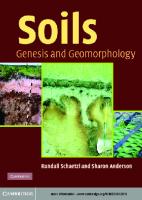
Figure 1.1 Examples of various soil types and profile morphologies from North America. (A) Paleustoll (Flatirons series) formed in alluvium on an early Pleistocene pediment in the Colorado Piedmont, just east of the Rocky Mountain front. The soil has a thick, dark, surface horizon high in organic matter (a mollic epipedon), classifying it as a Mollisol. The current climate is semiarid, with a spring-summer rainy season (ustic moisture regime). The soil has a very well expressed (deep reddish-brown, thick, clay-rich) argillic (Bt) horizon (with intensely weathered gravel), placing it in the “pale” Great Group. The scale is in feet. (B) Spodosol from the Upper Peninsula of Michigan, illustrating development of the E and Bhs horizons in sandy, glacial outwash. (C) Alfisol (Hapludalf) from southern Michigan illustrating development of A-E-Bt horizonation typical of postglacial soils in the area developed on loess and till (slide 1–6 from the Marbut Memorial Slide set, Soil Science Society of America; reproduced with permission of the Soil Science Society of America). Scales are in feet.

8

SOILS IN ARCHAEOLOGICAL RESEARCH

Hodgson (1997) presents the standards used in Great Britain (see also Catt, 1990), and Duchaufour (1998, pp. 146–147, 148) and van Breemen and Buurman (2002, pp. 141, 365–366) summarize the Food and Agriculture Organization of the United Nations (FAO-UNESCO) system (to be updated and superceded by the FAO World Reference Base for Soil Resources [FAO-WRB]; see Duchaufour, 1998, pp. 151–152) employed throughout continental Europe (see Driessen and Dudal, 1991). All of these sources also provide additional specifics on the terminology and data necessary to describe soils. Some additional nonstandard (i.e., non-USDA-approved) horizon nomenclature, developed by soil geomorphologists and Quaternary geologists, or by pedologists in other countries, is also provided in table 1.1 and discussed in appendix 1. The USDA horizon nomenclature, with modifications described in appendix 1, is used throughout this volume. Older or foreign nomenclatures used in sources for figures and tables were converted, unless noted. To fully understand late-20th-century and contemporary USDA-based pedology, the concept of the “pedon” must be noted. The pedon is the smallest body of one kind of soil large enough to represent the nature and arrangement of horizons (Soil Survey Division Staff, 1993, p. 18). Essentially, the pedon is the soil profile in three dimensions; a conceptual unit of soil defined for sampling purposes (see Schelling, 1970, p. 170; Buol et al., 1997, pp. 36, 43–44; Soil Survey Staff, 1999, pp. 10–14). Whereas the pedon is conceptual, the “soil individual” (or “polypedon”) is a real body of soil on the landscape (essentially, more than one pedon; Schelling, 1970, pp. 170–171; Buol et al., 1997, pp. 36–37). These terms and definitions are obscure and somewhat unfathomable, and the concepts have little relevance to geomorphology or geoarchaeology; they are mentioned because they are key concepts in USDA soil mapping (chapter 4). Soil Horizons versus Geologic Layers Soil horizons are not the same as geologic layers. Soil horizons form in geologic layers. Learning how to distinguish between soil horizons and unaltered sediments is another important step in learning how to recognize soils (Stein, 1985, p. 6; Mandel and Bettis, 2001b, p. 175). The use of the term “layer” interchangeably with “horizon” in some literature (including soil science publications) is particularly unfortunate and further confuses the issue of differentiating soils from sediments (Wilson, 1990, pp. 61–62, 71). Geologic layers follow the Law of Superposition: they are deposited one atop the other, with the bottom layer being the oldest and the top layer the youngest. Soil horizons are superimposed over, and thus postdate, the geologic materials in which they form (their parent material), and in general, horizons develop from the top of their parent materials downward (see chapter 5 and Cremeens and Hart, 1995). The boundaries between soil horizons, therefore, typically have no relationship to geological layering (discussed further in chapter 5). An individual soil horizon can form through several depositional layers, and conversely, several horizons can form within a single deposit. Distinguishing between horizons and geologic layers sometimes is difficult (discussed further in chapters 5 and 10), particularly given the heavy emphasis

INTRODUCTION

9

on stratification and superposition in the training of archaeologists as well as geologists (e.g., Tamplin, 1969, pp. 153–154; Wilson, 1990, pp. 61–62, 71). For example, a layer of organic-rich sediment subjected to bioturbation and burial may be confused with a buried A horizon (fig. 5.7). A zone of pedogenically translocated humus (Bh horizon), common in podzolizing environments, likewise may be misidentified as a buried A horizon. Conversely, Rutter (1978) recalled an incident in which an archaeologist described an A-Bw-Bk profile, subsequently identified by a pedologist as layers of peat, loess, and volcanic ash, respectively. Confusion of horizons for layers, and vice versa, can have profound consequences in interpreting landscape evolution, site formation, or cultural stratigraphy, as discussed in chapters 9, 10, and 11.

Soils in Geoarchaeological Research Soil science has its roots in both the geological and agricultural sciences (Tandarich, 1998a,b). This book is written largely from the geosciences perspective but also includes agricultural aspects that bear on the interpretation of the human past. Much of the volume deals with pedology. Though traditionally taught in agricultural schools, pedology is an earth science by virtue of its focus on soil in the context of landscape, surficial processes, and surficial deposits. The subdiscipline of pedology and geoscience that is most directly related to archaeology is soil geomorphology. In particular, much soil geomorphic research involves the study of soils in an attempt to reconstruct paleoenvironments and paleolandscapes or for dating (e.g., Ruhe, 1965; Boardman, 1985b; Jungerius, 1985; Richards et al., 1985; Knuepfer and McFadden, 1990; Gerrard, 1992; Birkeland, 1974, 1984, 1999) and thus has obvious archaeological implications. Geoarchaeologists K. Butzer (1982) and T. Van Andel (1994), a geographer and a geologist, respectively, suggest that one of the most significant aspects of geoarchaeological research is the analysis of landscapes, especially in terms of the changing options they present to their human occupants (Van Andel, 1994, p. 32; see also Fedele, 1976, and Gladfelter, 1977). Few aspects of the environment are as intimately linked to the landscape as soils, and thus, the appreciation and study of soils should be an integral component of geoarchaeology. Increased interest in soils and soil science applications in archaeology has followed the growth of geoarchaeology, which began more or less when the term “geoarchaeology” was coined (Butzer, 1973; Rapp et al., 1974). For example, in 1977 the Geological Society of America (GSA) established an Archaeological Geology Division; in 1986 the journal Geoarchaeology was inaugurated; in 1990 the GSA published a volume on the subject (Lasca and Donahue, 1990) as part of its Centennial series; and in 1992 M. R. Waters published the first single-author volume devoted exclusively to geoarchaeology (Waters, 1992). The study of soils as a component of geoarchaeology similarly evolved, though lagging somewhat behind the broader geoscientific aspects of archaeology. The late 1980s saw publication both of an edited volume devoted to anthropogenic soils (Groenman-van Waateringe and Robinson, 1988) and of the first volume on soil micromorphology in archaeology (Courty et al., 1989), followed by an issue of

10

SOILS IN ARCHAEOLOGICAL RESEARCH

World Archaeology (1990, v. 22, n. 1) on “soils and early agriculture” and the first edited volume on soils in archaeology (Holliday, 1992b). This trend continued through the 1990s and into the early 2000s. Almost half of the 35 papers in Lasca and Donahue (1990) deal directly or indirectly with soils. They are also a prominent component of subsequent edited volumes on geoarchaeology (Barham and Macphail, 1995; Goldberg et al., 2001; Stein and Farrand, 2001), including historical treatments (Mandel, 2000). In the meantime, archaeology emerged in mainstream soil science. Two international conferences on “pedoarchaeology” were held in 1992 (Orlando, Fla.; Foss et al., 1993b) and 1994 (Columbia, S.C.; Goodyear et al., 1997). Archaeology was featured prominently in two symposia at the annual meeting of the Soil Science Society of America in 1993, resulting in publication of an edited volume on pedology in archaeology (Collins et al., 1995). Furthermore, the role of soils in archaeological research (Holliday, 1994) was highlighted in a symposium honoring the 50th anniversary of Jenny’s (1941) “Factors of Soil Formation” (Amundson, 1994). Scudder et al. (1996) also produced a lengthy review paper on soil science and archaeology in an agronomy monograph series, which introduced the term “archaeopedology” (p. 6; along with Reitz et al., 1996, p. 5) without defining it. A telling example of the wide interest in the subject of soils in archaeology is in the disciplinary backgrounds of the investigators dealing with soils in Lasca and Donahue (1990), Holliday (1992b), Collins et al. (1995), and Goldberg et al. (2001): The authors include archaeologists, pedologists, geologists, and geographers. Such cross-disciplinary interests and interdisciplinary approaches significantly advance the field. Soil science, particularly pedology, and archaeology are closely allied in their temporal and spatial scales, and among the earth sciences, pedology is most similar to archaeology in scales of operation and process (Holliday et al., 1993). These similarities in scale are apparent in both regional and site-specific studies. At large (regional) scales, soil stratigraphy has long been used in archaeology for correlating sites and for dating (e.g., Leighton, 1937; Albritton and Bryan, 1939; Bryan, 1941a; Movius, 1944). Soil geomorphic investigations also are compatible in scale to regional archaeological investigations, focusing on dating, environmental reconstruction, and late-Quaternary landscape evolution (e.g., Dan et al., 1968; Dan and Yaalon, 1971; Gile et al., 1981; Pope and Van Andel, 1984; Grolier, 1988; Overstreet and Grolier, 1988, 1996; Blair et al., 1990; Fedele, 1990; Wells et al., 1990; Mandel, 1994; Brinkmann, 1996; Wilkinson, 1997; Belcher and Belcher, 2000). Soil micromorphology (soil petrography; see chapter 2) is also useful for regional geomorphic and archaeologic studies, including investigations of sediment provenance, landscape evolution, environmental reconstructions, and agricultural development (e.g., Courty et al., 1989; Courty, 1992, 2001). At small (site-specific) scales, the focus of pedology—the soil profile—is similar in scale to many archaeological sites (tens of centimeters to a few meters thick), and the scale of many pedological features is similar to that of archaeological features (a few millimeters to tens of centimeters thick; Holliday et al., 1993). Soil variability at small scales as a function of slope, drainage, or lithologic change is a common theme in pedology and is also of archaeological significance

INTRODUCTION

11

for stratigraphic correlation and interpretation of site formation processes. Temporal scales of formation of individual pedogenic versus anthropic features are disparate (centuries to millennia versus days to decades, respectively), but overall, processes of site formation and cultural evolution operate at temporal scales similar to those of soil formation (decades to millennia). The scalar compatibility of archaeology and pedology strongly argues for pedologists and pedologic perspectives to be involved in all phases of archaeological research (Holliday et al., 1993). Beyond the issue of scale, pedologists and archaeologists also share another important perspective: understanding the soil as a resource, now and in the past (Jacob, 1995b, p. 54). The agriculture tradition in pedology provides a unique perspective for archaeologists who are trying to understand the origins, evolution, and characteristics of agriculture. Pedologists can also provide important insights into understanding human effects, such as soil erosion, on soils. Soil stratigraphy and soil chemistry, rather than pedology and soil geomorphology, are perhaps the best-known and oldest applications of soil science in archaeology and also will be discussed in this volume. These two applications have very different disciplinary traditions, however. Soil stratigraphy has its origins in Quaternary geology, in which soils have long been recognized as stratigraphically and paleoenvironmentally significant (Leverett, 1898; Leighton, 1937, 1958; Bryan, 1941a, 1948; Bryan and Albritton, 1943; Ruhe, 1965; Haynes, 1968; Valentine and Dalrymple, 1976). Quaternary geologists and geomorphologists working with archaeologists were quick to recognize soils in stratified archaeological contexts and to use the soils as clues to past environments (e.g., Leighton, 1936; Bryan, 1941a; Haynes, 1968; Antevs, 1941). Paleontology and paleobotany (especially palynology) were important components of such research, but the physical and chemical characteristics of the soils themselves seldom were discussed or dealt with. Soil chemistry has long been studied both by soil scientists and archaeologists for clues to human impact on the landscape, especially for reconstructing agricultural activity and for detecting human occupation (e.g., Arrhenius, 1931, 1963; Solecki, 1951; Cornwall, 1958; Berlin et al., 1977; Eidt, 1977, 1984, 1985). Soils as pedologic entities, however, often are unrecognized or not dealt with in these studies. R. C. Eidt (1984, 1985), a geographer, is one of the few scientists to combine traditional pedologic approaches with soil chemistry to investigate anthropogenically modified soils (“anthrosols”; further discussed in chapter 11). The historic dichotomy in the use of soils for stratigraphic or paleoenvironmental purposes versus their use as keys to anthropogenic impacts on the landscape also has a rough geographic separation. Most research on soils in archaeological contexts has taken place in North America and Europe. Many of the North American studies focused on soils as stratigraphic markers and as age and paleoenvironmental indicators, as is the case in the loess-rich areas of Europe. Outside these areas in Europe, however, and most notably in Great Britain, the research emphasis tended to be on the use of soils as indicators of human impact or human paleoenvironments (though rapid growth in these areas of interest began in the 1970s in North, Central, and South America, e.g., Eidt and Woods, 1974; Woods, 1975, 1977, 1984; Eidt, 1984, 1985; Sandor et al., 1986;

12

SOILS IN ARCHAEOLOGICAL RESEARCH

Sandor, 1987; Dunning, 1994). This regional variation probably is a result of differences in the nature of the archaeological record in the two regions and in the history of geoarchaeological research in each. In North America, archaeological sites with long records of human occupation in thick, well-stratified deposits with intercalated buried soils are relatively common, especially in the central and western regions. The impact of prehistoric peoples on soils and on the landscape was minimal, however. In Europe, in contrast, humans exerted a profound effect on the landscape for thousands of years. These effects have long attracted the attention of archaeologists and geoscientists, whose geographically distinct approaches to soils applications in archaeology can be seen in some of the earliest systematic treatments of soils as clues to the past (compare the North American perspectives of Bryan [1948] and Bryan and Albritton [1943] with the British approach of Cornwall [1958, 1960]) and are readily apparent by comparing the papers on North American archaeological sites in Lasca and Donahue (1990), Holliday (1992b), and Collins et al. (1995) with the studies from northern Europe and Great Britain in the papers assembled by Groenman-Van Waateringe and Robinson (1988) and Barham and Macphail (1995) and in the comprehensive works of Cornwall (1958) and Limbrey (1975). Soil geomorphology, with the landscape at its core, provides an integrative link between soil stratigraphy, pedology, and soil chemistry and their applications in archaeological and geoarchaeological research. In this volume, a soil geomorphic approach is used to assess soil surveys (chapter 4) and to link studies of soils as stratigraphic markers (chapters 5, 6), as age and paleoenvironmental indicators (chapters 7 and 8), as clues to landscape evolution and site formation processes (chapters 9 and 10), and for the study of anthropogenic soils and human effects on the environment (chapter 11). Each chapter includes a discussion of basic principles and their archaeological implications and a presentation of case histories.

2

Terminology and Methodology

The long history of soil science (e.g., well over 100 yr in North America) and its bureaucratic institutionalization as a component of agricultural research in many countries resulted in the evolution of a substantial vocabulary and methodology for the discipline. A wide array of methods for the field and laboratory investigation of soils also is available to geoarchaeologists. The first part of this chapter is a discussion of some basic terms and definitions used in pedology and soil geomorphology. Some specific terms (e.g., soil stratigraphic nomenclature) are discussed as necessary elsewhere in the text and in appendix 1. There is a sizable body of nomenclature in pedology and soil geomorphology for describing and classifying soils. Indeed, there is a tendency in soils research toward an overabundance of nomenclature and jargon (e.g., Fastovsky, 1991). All scientific fields necessarily have a specialized nomenclature, however. Researchers in any field, and especially interdisciplinarians such as archaeologists working with soils and soil scientists working with archaeology, should be aware of the nomenclature, jargon, and lingua franca of the new fields they enter. A pedologist who becomes involved with North American archaeology would have to become familiar with terms and concepts such as “Paleoindian” or “Archaic” or “site.” Likewise, archaeologists and geoscientists interested in understanding soils for geoarchaeological purposes must learn some basic soil science terminology and the principles behind issues of proper use (or misuse) of some terms. This fosters communication and problem solving and avoids ambiguities. The rest of this chapter is a discussion of some of the more widely used approaches in the field and in the laboratory, especially in archaeological contexts. Key points to be made are that, first, investigators select the methods that 13

14

SOILS IN ARCHAEOLOGICAL RESEARCH

best suit the field situation and the research questions being posed; second, if comparisons are made to other research, the comparable methods should be used; and third, all field and laboratory methods should be referenced in publications and deviations from standard practices or procedures should be described.

Nomenclature and Definitions Some terms introduced below and elsewhere are well defined and generally agreed on, whereas others are variously or vaguely defined. There are also variations in terms and nomenclature from country to country because much of the jargon was devised by or developed under the direction of the agricultural agencies of national governments for the mapping, classification, and management of farm land or other aspects of land use. The history of some of the terms (and the ensuing confusion over meanings) is discussed by Johnson and Hole (1994), and varying applications (and definitions) of the terms are well illustrated among the papers collected and edited by Follmer et al. (1998). Some of the more useful international terminology is discussed in the text (especially chapter 5) and in appendix 1. Soil Classification An important component of pedology is soil classification, which is the categorization of soils into groups at varying levels of generalization according to their morphological and chemical properties and sometimes their assumed genesis (Buol et al., 1997, p. 5). The purpose of classification is systematizing knowledge about soils and determining the processes that control similarity within a group and dissimilarities among groups (Birkeland, 1999, p. 29). The classification system used in the United States is the U.S. Comprehensive Soil Classification System, or “soil taxonomy,” published as Soil Taxonomy (Soil Survey Staff, 1975, 1999; www.soils.usda.gov). This system often is incorrectly referred to as the “7th Approximation” (the title of an earlier version of the classification system [Soil Survey Staff, 1960; see Soil Survey Staff, 1975, preface]). The U.S. system was developed in the 1950s and 1960s and was a revolutionary concept in soil classification. Most earlier schemes were based in large part on the presumed genetic history of the soils (e.g., red desert soil, brown forest soil)—which is almost never immediately apparent—and on nonsoil characteristics (e.g., local vegetation or groundwater level) rather than on properties of the soils themselves. In addition, many of the terms used in the earlier systems derived from various foreign languages, folk terms, and coined names; were generally poorly defined; and were not always mutually exclusive (Butler, 1980, pp. 72–74; Buol et al., 1997, pp. 222–223). The newer U.S. system is an approach to soil classification based entirely on the soils as they are, relying on properties observable in the field or measurable in the laboratory (Soil Survey Staff, 1975, 1999; Bartelli, 1984). To appreciate the applications and limitations of soil taxonomy in archaeological and geoscientific research, the purpose of the system must be fully

TERMINOLOGY AND METHODOLOGY

15

understood. An explanation of soil taxonomy is facilitated by contrasting it with what it is not. Soil taxonomy was designed to facilitate classification for soil survey and land-use purposes (Soil Survey Staff, 1975, pp. 7, 8; Bartelli, 1984) and is geographically biased toward the agriculturally productive soils of the midlatitudes. It was not designed to be a tool in soil geomorphic or other geoscientific research. The Soil Survey Staff (1975, p. 7; 1999, p. 15) describes the primary objective of soil taxonomy as having “hierarchies of classes that permit us to understand, as fully as existing knowledge permits, the relationships between soils and also between soils and the factors responsible for their character.” Bartelli (1984, p. 9), in discussing the development of soil taxonomy, further notes that observable or measurable soil properties were selected to group soils of similar genesis. Soil taxonomy is arguably at odds with these objectives, however. The system does not provide a means of understanding relationships between soils beyond their spatial relationships on soil maps, and it is also largely divorced from the factors of soil formation (viewed as both an advantage and disadvantage of the system; see Morrison, 1978; Birkeland, 1999; Holliday et al., 2002). The development of soil taxonomy involved essentially no research into the genetic relationships among soils, and very little soil survey research in the United States has focused on the genesis of soils or soil mapping units (Holliday et al., 2002). Examples of these aspects of soil taxonomy as manifested in soil surveys are explored in chapter 4. Furthermore, and of particular significance to geoarchaeology, soil taxonomy is not well suited for application to buried soils (discussed below and in chapter 5) and inadequately deals with soils heavily altered by human activity (so-called “anthrosols,” discussed below and in chapter 11). Finally, soil taxonomy is not an exhaustive inventory of all known soils or pedogenic relationships. This is an important consideration when using soils, either at the surface or buried, for reconstructing the past. Some assume or imply that soil taxonomy represents the universe of soils and that interpretation is simply a matter of picking out the correct soil or soils from those listed (e.g., Smith and McFaul, 1997, p. 130; Retallack, 2001), but most of the soils listed in taxonomy at the suborder level are soils that have been investigated, to some degree, largely in the United States. Undoubtedly, many more variants (both in the United States and, particularly, around the world) await description and classification. The U.S. soil classification system is based on a variety of differentiating characteristics including diagnostic horizons (table 2.1) and related properties, such as soil moisture and soil temperature. The terms for the different characteristics were derived from Greek and Latin roots. The diagnostic horizons and other characteristics are strictly defined and based on measurable soil properties and, therefore, convey a wealth of data. The diagnostic horizons are not the same as the more generally defined A-B-C horizon symbols used in field descriptions, although there is often a general correlation (table 2.1). The mollic epipedon, for example, is a surface horizon identified on the basis of thickness, Munsell color, organic carbon content, and citrate-extractable phosphorus content, among other characteristics. It may or may not be the equivalent to the A horizon (e.g., it may include the A and upper B horizon). In contrast, the A horizon is a field designation for a horizon found at the surface or below an O horizon and characterized by humified organic matter mixed with mineral material.

16

SOILS IN ARCHAEOLOGICAL RESEARCH

Table 2.1. General concepts for selected diagnostic horizons in soil taxonomy Epipedons (Diagnostic Surface Horizons) Anthropic Histic Mollic Ochric Plaggen

Mollic epipedon high in phosphorous content Surface horizon very high in organic matter (O) Deep, dark, humus-rich surface horizon with abundant cations (A, A&B) Surface horizon that does not meet the qualifications of any other epipedon (A) An artificially made surface layer produced by long-term manuring

Diagnostic Subsurface Horizons Albic Argillic Calcic Cambic Kandic Natric Oxic Petrocalcic Spodic

Light-colored horizon with significant loss of clay and free iron oxides (E) Horizon of significant clay accumulation (Bt) Horizon of significant accumulation of calcium carbonate (Bk) Some reddening or structural development; reorganization of carbonates if originally present (Bw) Heavily weathered, clay-rich horizon low in bases (Bt) Argillic horizon high in sodium (Btn) Intensely weathered horizon virtually depleted of all primary minerals and very low in bases Calcic horizon strongly cemented by calcium carbonate (km or K) Horizon of significant accumulation of aluminum and organic matter with or without iron (Bh, Bs, Bhs)

These are very general definitions of terms used in the soil classification system of the U.S. Department of Agriculture (based in part on Wilding et al., 1983a). Considerable field and laboratory data are necessary to determine diagnostic horizons. For a complete list and criteria see Soil Taxonomy (Soil Survey Staff, 1999). Diagnostic horizons are not exact equivalents of field designations (e.g., not all Bt horizons are argillic horizons), although there is a general relationship. Some probable field equivalents are given in parentheses.

The classification system is hierarchical with six categories (from general to specific): order (table 2.2), suborder, great group, subgroup, family, and series. A formative element of the term used at each higher category is carried down through successive lower categories to the great group level (fig. 1.1A). For example, the Flatirons series is a Mollisol in an ustic moisture regime with a well-expressed argillic horizon, classifying it in the Paleustoll great group (fig. 1.1A). The subgroup is written as two words. In the case of the Flatirons soil, it is in a dry setting and therefore identified as an Aridic Paleustoll. Families differentiate the subgroups on the basis of physical and chemical characteristics such as texture, mineralogy, and temperature. The Flatirons soils are clayeyskeletal, smectitic, mesic Aridic Paleustolls. The soil series is the basic unit of soil mapping (further discussed in chapter 4). The series represents the grouping of soils with similar profile characteristics within a given region. Soil series are typically named after places, and usually a town. For soil geomorphological and geoarchaeological research, an understanding of the classification to the great group or possibly subgroup level probably is sufficient and, in any case, more meaningful than the family and series nomenclature (further discussed in chapter 4). The terms used in U.S. soil taxonomy are many and are strictly defined (tables 2.1, 2.2). Many of these terms and their definitions appear unusual and confusing at first, but with experience, researchers should find them quite usable and

TERMINOLOGY AND METHODOLOGY

17

Table 2.2. General concepts of the soil orders in soil taxonomy Term

Definition

Alfisols

Soils with argillic horizon, but no mollic (A-Bt), that are lower in bases than Mollisols; typically found in humid, temperate regions Soils formed in volcanic ash and related volcanic parent materials (A-C, A-Bw) Soils formed in desert conditions (Entisols can also be found in deserts) or under other conditions restricting moisture availability to plants (high salt content; soils on slopes); with or without argillic horizon, but commonly with calcic, gypsic or salic horizons (A-Bw-Bk; A-Bt-K; A-By) Soils with little evidence of pedogenesis (A-C, A-R); very few diagnostic horizons Permafrost soils; very common in high latitudes Organic soils, such as peats Soils exhibiting more pedogenic development than Entisols, with appearance of diagnostic surface and subsurface horizons that are not as well developed as in most other orders (A-Bw) Soils with a mollic epipedon and high in bases throughout; typical of continental grasslands Soils with an oxic horizon; found in tropical regions and include many soils formerly termed Laterites and Latosols Soils with spodic horizons (O-A-E-Bh/Bs/Bhs); typical in cool, humid climates under coniferous forests Highly weathered soils that have argillic horizons and that are very low in bases (A-Bt); typically found on older landscapes in warm, humid climates Soils high in clay content in climates with distinct wet and dry seasons and that shrink and swell markedly

Andisols Aridisols

Entisols Gelisols Histosols Inceptisols

Mollisols Oxisols Spodosols Ultisols Vertisols

For a complete list and criteria see Soil Taxonomy (Soil Survey Staff, 1999). To properly classify a soil one must follow the guidelines and criteria for diagnostic horizons and classification in soil taxonomy (Soil Survey Staff, 1999). This table presents only the principal characteristics of the soil orders.

useful. Buol et al. (1997) provide a good introduction to soil classification, but formal instruction is especially recommended. The U.S. soil classification system has been compared to hierarchical biological classification (e.g., Retallack, 1990, p. 91). As pointed out by Fitzpatrick (1971), however, most soil classification systems are hierarchical, yet there is no reason to assume that soils are genetically related in the manner that they are grouped into hierarchies. Soil classifications are developed for a variety of purposes and are imposed on a natural system. Most soil classification schemes, such as soil taxonomy, are designed for agricultural and other types of land use, not for interpreting landscape evolution or human history. This particular aspect of soil taxonomy seems to be poorly understood by many geoscientists. Soil taxonomy has been criticized by some—geologists and soil geomorphologists in particular (e.g., Hunt, 1972; Morrison, 1978; Holliday et al., 2002), but also pedologists (e.g., Fitzpatrick, 1971, 1979). Hallberg (1984) provides an excellent overview and critique of soil taxonomy from the perspective of a geologist. Most problems in the classification system stem from the need for arbitrary rules or decisions inherent in any attempt to categorize and classify parts of a continuum. As Hallberg (1984, p. 53) notes, “classification involves . . . the Tyranny of the Pigeonhole.” He further points out that, “the institutional, or bureaucratic

18

SOILS IN ARCHAEOLOGICAL RESEARCH

implementation of the U.S. system of soil taxonomy . . . has often had the effect of making [it] inflexible; its implementation often rigid and legalistic” (Hallberg, 1984, p. 57). In other geosciences, in contrast, there are a number of “scientific codes or guidelines put forth by professional societies, which are freely debated in the scientific literature [and at] professional meetings,” (Hallberg, 1984, p. 57) such as the Code of Stratigraphic Nomenclature (e.g., North American Commission on Stratigraphic Nomenclature [NACOSN], 1983), in geology (further discussed in chapter 5). Because many soil geomorphologists are trained in geology or physical geography they often alter terms from the soil taxonomy to suit their needs. For example, they provide adjectives such as “weak argillic horizon” (Btj or juvenile Bt in field nomenclature) for horizons that barely meet argillic criteria (Birkeland, 1999). This can be a very useful approach in soil geomorphic and geoarchaeological research, and a number of nonstandard terms are used in this volume (see further discussion and appendix 1). More specifically, much of the criticism of soil taxonomy is aimed at the terminology introduced, the absence of genetic information in the system, and the difficulties in applying the system to buried soils. The last point is of concern in soil geomorphic studies, but much of the basic terminology of soil taxonomy remains useful in such circumstances even if full classification is not. Some of the classificatory terms do appear odd at first, but they are simply not that difficult to learn. Once the basic diagnostic terms are understood, a vast number of classificatory words can be put together, and a single word will then carry a large amount of qualitative and quantitative information (fig. 1.1A). Moreover, the system is used by most individuals doing the basic soils research (in both academic and governmental contexts) in the United States, and therefore any investigator interested in soils in the United States must become familiar with the system to understand the literature. Beyond the pros and cons of the basic concepts behind soil taxonomy and its terminology, the system is difficult to apply to buried soils (Mack et al., 1993; Nettleton et al., 1998; Holliday et al., 2002; see also the discussion of buried soils in chapter 5). Applying both the diagnostic horizon nomenclature and taxonomic classification to buried soils is problematic because of either the erosion of nearsurface horizons or the postburial alteration of the soils (chapters 5, 10), both of which are greater the longer the soil or sediment has been buried, and because soil taxonomy is explicitly designed for surface soils. Components of buried soils can be described in terms of diagnostic horizons, but the characteristics of the horizon may be different from its preburial state. Erosion or compaction changes horizon thickness, for example, which is a significant component of the requirements for a mollic epipedon and a calcic horizon (table 2.1). The color of a mollic epipedon, also a classificatory requirement, usually changes after burial because of oxidation of organic matter. Furthermore, pedogenesis in the deposits that bury a soil may modify the buried soil in a process known as “soil welding” (Ruhe and Olson, 1980; also see chapter 5): a calcic or argillic horizon can be superimposed over a buried mollic epipedon or argillic horizon, for example. Taxonomic classification of a buried soil often is possible if a complete buried profile is preserved and the burial was recent, but the classification will differ from the preburial classification over the long term. Burial changes characteris-

TERMINOLOGY AND METHODOLOGY

19

tics of the diagnostic horizons and almost always changes soil moisture and soil temperature—environmental characteristics necessary for much classification. Significant changes in soil and water chemistry can also accompany or follow burial and can significantly affect classificatory characteristics such as base saturation. Further problems can be encountered when classifying buried soils in terms of horizons and taxonomy for paleoenvironmental interpretations because few types of horizons or taxonomic categories are associated with unique environmental conditions (e.g., Dahms and Holliday, 1998), an issue further explored in chapter 8. Because of the difficulty of applying soil taxonomy to the classification of buried soils, especially pre-Quaternary soils, alternative classifications have been proposed (Mack et al., 1993; Nettleton et al., 1998, 2000). Interestingly, they use terms, concepts, and a structure from or similar to that of soil taxonomy. The determination of which system, if any, becomes the lingua franca in studies of buried soils awaits extensive field testing. Knowing how to describe or classify a soil is only the first step in using soils in archaeology or soil geomorphology. Such knowledge is only a tool for communication and interpretation. The number of archaeological site reports with descriptions and classifications of soils, but no further discussion of them, indicates that this aspect of recognizing and classifying soils is poorly understood by many archaeologists (and some collaborating soil scientists and geologists). Recognizing soil horizons or classifying a soil is a very basic first step in the geoarchaeological interpretation of a site, akin to learning pottery types or recognizing flaking patterns on stone tools as a step toward reconstructing human behavior. Working outside of the United States, researchers may want to become familiar with other classification systems. Some are similar to soil taxonomy, but others are not. Lof (1987) provides a useful correlation and comparison, with color photos, of the FAO classification scheme with those of the United State, Canada, England and Wales, France, Germany, and Australia. Comparisons of the structure, philosophy, advantages, and disadvantages of a variety of soil classification systems, including soil taxonomy, are provided by the Soil Survey Staff (1975, pp. 437–455), Butler (1980, pp. 72–122), and Buol et al. (1997, pp. 195–233). The International Institute for Geo-Information Science and Earth Observation (ITC), in The Netherlands, prepared a very useful “Compendium of On-Line Soil Survey Information” including information on and comparisons of the major national soil classification systems (www.itc.nl/~rossiter/research/rsrch_ss_class.html). Other Terms Beyond the “official” governmental soils nomenclature, a variety of informal terms is used in the more geologically focused studies of soils such as soil stratigraphy and soil geomorphology, and in the more archaeologically focused work in geoarchaeology. The following section is a discussion of the more widely used terminology from these fields. Some other, specific soil geomorphic terms are introduced in chapter 3. The specifics of soil stratigraphic terminology are reviewed in chapter 5.

20

SOILS IN ARCHAEOLOGICAL RESEARCH

The term “paleosol” is widely used in archaeology and other Quaternary studies and is variously defined. These definitions include soils of obvious antiquity (Morrison, 1967, p. 10), ancient soils (Butzer, 1971, p. 170), soils formed on a landscape of the past (Ruhe, 1965, p. 755; Yaalon, 1971c, p. 29; Gerrard, 1992, p. 202; Catt, 1998) or under an environment of the past (Yaalon, 1983), a soil with distinct evidence that the direction of soil development was different from that of the present (Catt, 1998), a soil formed during an earlier period of pedogenesis (Allaby and Allaby, 1991), or soils formed under conditions generally different from those of today (Plaisance and Cailleux, 1981, p. 702). Specific types of paleosols include “buried soils,” which are soils covered by sediment (figs. 2.1–2.3, 6.4, 6.14, 6.18, 6.20, 6.21, 7.6, 7.11, and 8.4–8.6);“relict soils,” which are soils formed on past landscapes or under past environments and never buried; and “exhumed soils,” which are soils that were buried and subsequently re-exposed (Ruhe, 1965; Valentine and Dalrymple, 1976; see Johnson and Hole [1994] and chapter 5 for further discussion of these terms). Among these terms, “buried soil” is probably the least ambiguous, although a distinction between a buried soil and a buried paleosol is proposed (Catt, 1998, p. 84). The former term is used for “soils buried by deposits too thin to seal them from present pedogenesis and not showing evidence of development in a direction different from the present,” and the latter term is proposed for soils that are buried and “isolated from present pedogenesis” or soils that are buried and exhibit “distinct evidence that the direction of soil development was different from that of the present.” Otherwise, among the definitions and types of paleosols, exactly what constitutes a past landscape or past environment or how old the soil has to be was never defined. Because landscapes always are being subjected to some modification and the environment is never static, and because all soils take some time to form, arguments have been made that all soils are paleosols and all unburied soils are relict soils, making such terms redundant (see also Bos and Sevink, 1975; Fenwick, 1985; Johnson et al., 1990; Bronger and Catt, 1998a,b; Follmer, 1998; D. L. Johnson, 1998; Johnson and Hole, 1994). Moreover, these definitions require that the history of the soil, the landscape, or both be known before the term can be applied. In any case, there seems to be no reason to differentiate soils based on their relevance to the past or present. In geology, a gravel layer is a gravel layer, whether it was deposited in this century or in the Permian. If the gravel is lithified then it is a conglomerate, but otherwise no distinction is necessary. The term “paleosol” seems to have some utility, however, judging from its widespread use (e.g., Follmer et al., 1998), especially in dealing with soils in the rock record— so-called pre-Quaternary soils (e.g., Retallack, 1990). The following criteria and definitions, based largely on the author’s experience and views, may clarify the differentiation of soils, buried soils, and paleosols. A soil, as defined previously, can be a recently formed unburied soil or deeply buried soil from the Triassic. Age, genesis, and stratigraphic position are irrelevant. A “ground soil” or “surface soil” refers specifically to unburied soils. A “buried soil” is any soil in which sediments cover a clearly recognizable horizon sequence, regardless of the thickness of the cover sediments (see also the definition of an “isolated paleosol” by Schaetzl and Sorenson [1987]). A paleosol is a

Figure 2.1 Buried soils at the Lubbock Lake Site, Texas. (A) Good example of the late Holocene soil sequence (Trench 95, with a profile picked out by a knife). The b3 is the Lubbock Lake soil, formed in stratum 4B ~4500–1000 yr B.P., then buried by stratum 5A. The carbonate in the Bkb3 horizon probably is from the b2 soil (lower 5A), providing a nice illustration of soil welding. The Apache soil (b1) formed in upper 5A. The weakly expressed surface soil is the Singer Soil, formed in stratum 5B. (B) Cumulic facies of the Lubbock Lake soil in a lowland valley-axis position (Trench 141). The Btkb1, Btb1, and Btk’b1 horizons are soil stratigraphic equivalents of the Bkb3-Btb3Btkb3 in (A). The lower ABt probably was the original A horizon. It was cumulized by slowly aggrading mud of stratum 5 m (a lowland, muddy, valley axis facies of 5A) and eventually evolved into a Bt horizon. Thus, the cumulic A-ABt horizons in the lowland setting are a facies of the b2, Apache, and Singer soils more common in valley margin positions (fig. 2.1A).

A

B Figure 2.2 Buried soils in alluvium. (A) Fluvent in the floodplain of the Brazos River, northcentral Texas. Multiple thin, dark, buried A horizons (Ab) are apparent, in contrast to the lighter color of the unaltered alluvium. (B) Buried soils developed in alluvium at the Alum Creek site, central Kansas (Mandel and Bettis, 2001b, fig. 7.3; from Earth Sciences and Archaeology, by P. Goldberg, V. T. Holliday, and C. R. Ferring, © 2001, Kluwer Academic/Plenum Publishers. Reproduced with permission of Kluwer Academic/Plenum Publishers and R. D. Mandel). A relatively thin and weakly expressed buried A horizon is apparent above the shovel handle. The shovel is resting against a dark, cumulic A horizon. Note the sharp upper boundaries of the two buried A horizons in contrast to their more gradual lower boundaries (and compare with the abrupt lower boundary of the organic-rich deposit illustrated in fig. 5.7). Photo provided by and reproduced with permission of R. D. Mandel.

Figure 2.3 A very strongly expressed Bt horizon (with Bk horizon immediately below, and a less well expressed Bt below that) buried in fine-grained Pleistocene alluvium in southeastern Arizona. The A horizon is missing, probably because of oxidation and perhaps erosion. Note the very strong development of prismatic structure and the sharp upper boundary, but more gradual lower boundary.

23

24

SOILS IN ARCHAEOLOGICAL RESEARCH

soil that is both buried and lithified. This definition is relatively unambiguous and generally easy to apply in the field on visual examination. A related term that has some utility but is now out of favor is “fossil soil.” The term was essentially synonymous with buried soil until the mid-20th century (Johnson and Hole, 1994). Subsequent usage of the term was somewhat muddled, however, and it has largely disappeared from the literature. Fossil soil is a useful concept, though, as it refers to something that was once living and is now dead and buried or, using a broader definition of fossil (as an adjective), as something that existed in the geologic past and of which there is still evidence (Bates and Jackson, 1980, p. 243). Morrison (1978, p. 100) seems to equate buried soils with bisequums. A bisequum, however, refers to a pair of genetically related sets of illuvial B horizons with overlying eluvial horizons—typically an E-Bs sequum overlying an E¢-Bt sequum (Schaetzl, 1996, p. 23). By definition, a bisequum is a single soil. The terms “monogenetic” and “polygenetic” soils were coined by Bryan and Albritton (1943) based on geoarchaeological research in west Texas. A monogenetic soil was initially defined as “one developed in one climatic regime,” and a polygenetic soil was defined as having “developed in more than one climatic regime” (Bryan and Albritton, 1943, table on p. 477). Catt (1998, p. 84) provides more up-to-date definitions. A monogenetic soil “formed in a period when the variation in environmental factors was too small to produce detectably different assemblages of soil features . . . (i.e., the direction of soil development was constant).” A polygenetic soil “formed in two or more periods when the environmental factors were sufficiently different to produce detectably different assemblages of soil features . . . (i.e., the directions of soil development were different in the periods involved).” Similar to the criticism of the term and concept of paleosol (vs. soil), some argue that there is no such thing as a monogenetic soil and that all soils are polygenetic because environmental factors are always changing to some degree (e.g., Yaalon, 1971a, p. 155; Johnson et al., 1990; Johnson and Hole, 1994; D. L. Johnson, 1998). With the emphasis now placed on the direction of pedogenesis and the detectability of evidence for these changes, the terms may have merit and utility. This is clearly indicated by the concept of the “vetusol,” described next. Vetusol is a more clearly defined term that provides an important addition to concepts of buried soils and what they may tell us about environmental change. It refers to soils that evolved under the same or similar processes from their inception to the present time (Cremaschi, 1987). The term can be applied to a surface soil or a buried soil or both. For example, Busacca and Cremaschi (1998) describe a surface soil and as many as six buried soils that comprise a single vetusol. The point is that vetusols developed “under the influence of a single set of major pedogenic processes throughout their history and that they reacted only slightly to Pleistocene environmental changes” (Busacca and Cremaschi, 1998, p. 96). A vetusol, then, could be considered a kind of monogenetic soil that also represents long-term pedogenesis. The study of paleosols/buried soils often is referred to as “paleopedology” (Yaalon, 1971b; Retallack, 1990; Follmer, 1998). As with “paleosol,” this term seems to be very popular and is widely used, but its real utility is questionable.

TERMINOLOGY AND METHODOLOGY

25

In a broad, holistic sense, the study of buried soils, including paleosols, is a component of pedology, soil-geomorphology, and soil stratigraphy. As noted, however, pedology as traditionally taught in the United States does not deal with buried soils, and thus, some workers have found it necessary to use the term paleopedology, essentially to differentiate a geoscientifically based study of soils from an agricultural one. “Catena” is another important term in soil geomorphology because it describes a fundamental and significant aspect of soils (noted in chapter 5 and more fully discussed in chapter 9). As originally proposed (Milne, 1935a,b), a catena is a mapping unit defining a group or pattern of soils along a slope formed as a result of differential drainage on the slope, solute leaching down-slope, and erosion and deposition along the slope. In the United States, however, the term came to be applied to a sequence of soils developed in uniform parent material on a hill slope that vary according to drainage (fig. 2.4; Soil Survey Staff, 1951, p. 160). The term is often used interchangeably with “toposequence” (a group of soils that vary only in their topographic position; they otherwise formed in the same parent material, under the same climate and vegetation, and for the same amount of time; discussed in chapter 3) (Jenny, 1980, p. 280; Hall, 1983, p. 124; Buol et al., 1997, pp. 154–155; Birkeland, 1999, p. 235). The processes of erosion and deposition inherent in the formation of catenas mean that the age of the landscapes will vary, however (figs. 2.4 and 9.1). So even following the Soil Survey Staff approach, only some catenas are toposequences, and only some toposequences are catenas. In this volume the term catena is used more in the sense of Milne’s original concept. Related to catena is the concept of the “soilscape.” A soilscape is the pedologic portion of the landscape (Buol et al., 1997, p. 383) or the pattern and dis-

Figure 2.4 Schematic diagram illustrating geomorphic and pedogenic processes along a hypothetical catena (based on Birkeland et al., 1991, fig. 5.1, and Birkeland, 1999, fig. 9.2). Slope positions are: Su = summit, Sh = shoulder, Bs = backslope, Fs = footslope, and Ts = toeslope.

26

SOILS IN ARCHAEOLOGICAL RESEARCH

tribution of soils across the landscape. In a sense, soilscapes represent the expansion or distribution of catenas across the landscape. Catenary relationships among soils on a slope and the distribution of catenas across soilscapes are unique characteristics of soils as they form on and across landscapes and serve to distinguish soils from other geologic phenomena. The terms “anthrosol,” “anthropic soil,” or “anthropomorphic soil” have been around since at the least the mid-20th century (e.g., Soil Survey Staff, 1951, p. 133; Bunting, 1965, p. 131), but became popularized by Eidt (1977, 1984, p. 23). He initially defined anthrosols as “settlement-affected soils” (Eidt, 1977, p. 1327), and later as soils “whose native traits have been significantly altered by human activities” (Eidt, 1984, p. 23). Simple physical changes of a “native soil” resulting from human activity do not seem to be enough to qualify the soil as an anthrosol. In the examples discussed below and in most of the other literature on this topic, soils identified as anthrosols typically had significant chemical inputs as well as obvious physical changes resulting from human activity. In any case, the term “anthrosol” is now part of the general parlance and is used more broadly than Eidt probably intended. Some refer to purposely altered soils as anthrosols and use the term interchangeably with anthropogenic (e.g., Smith, 1980). In contrast, in the FAO-UNESCO (1994, p. 61) soil classification system, anthrosol is one of the major soil groupings for a broad array of soils “in which human activities have resulted in profound modification or burial of the original soil horizons.” Specific types of anthrosols in the FAO-UNESCO scheme include those subjected to deep cultivation, to long-term manuring, and to burial from long-term irrigation and from urban spoil. The FAO definition does not seem entirely satisfactory, however, because it could also include soils buried under mounds or tells or soils buried because of human-induced soil erosion. Few geoarchaeologists would consider those soils as anthrosols. Yet another use of the term is for soils that formed in anthropogenic sediments, but that do not necessarily display any indication of human effects on pedogenesis (e.g., Overstreet et al., 1988; Brinkmann, 1996; Overstreet and Grolier, 1996). This is not a widely used definition and is perhaps overly broad. The heart of the other definitions is that the soil itself is altered by human activity. Eidt (1984, p. 23) further subdivides anthrosols into “anthropogenic” soils, which were intentionally altered, and “anthropic” soils, which were unintentionally altered. Establishing the intent of ancient occupants of a region is difficult to do, but there are several kinds of soils that almost certainly were purposefully modified (e.g., the “plaggen” and “terra preta” discussed in chapter 11), as well as soils on many different landscapes that were artificially altered, but not with the intent of making specific changes. “Anthropogenic” literally refers to having an origin stemming from human factors. An anthrosol, therefore, is the result of anthropogenic processes. Distinguishing an “anthropogenic soil” as a type of anthrosol seems to serve no useful purpose. The term “anthropic” also has meanings that vary from Eidt’s definition. “Anthropic” is most widely used as a component of the U.S. soil taxonomy as a particular type of surface horizon. The “anthropic epipedon” is similar to the mollic in requirements for color, thickness, and organic carbon content, but it has a higher content of P2O5 because of “longcontinued use of the soil by humans, either as a place of residence or as a site for

TERMINOLOGY AND METHODOLOGY

27

growing irrigated crops” (Soil Survey Staff, 1999, p. 22), although little chemical or archaeological data are available for these horizons (e.g., Pettry and Bense, 1989). In this volume the term “anthrosol” is used to refer to soils that exhibit anthropogenic physical and chemical alterations. Soils subjected solely to chemical or physical alterations generally are not considered anthrosols, though some exceptions could be made.

Describing Soil Development In discussing soils, particularly in terms of their age or for making stratigraphic comparisons or correlations, describing the relative degree of soil development or pedogenic expression often provides a useful shorthand. Formal classification is often cumbersome and overly detailed for general comparisons, and many classification schemes are not designed to distinguish between degrees of soil development. For example, in soil taxonomy, horizons that qualify as argillic or calcic can vary significantly in their degree of development and morphological expression. In view of this situation a variety of informal terms are used to distinguish between soils based on overall degree of development. The following is one of the more widely used qualitative schemes for describing the degree of soil development (from Retallack, 1990, table 13.1; Birkeland, 1999, pp. 19–20), incorporating the well-known system for describing stages of carbonate accumulation (after Gile et al., 1966, and Machette, 1985; see fig. 3.3): A very weakly developed soil is one with an A horizon and perhaps a Cox horizon. If pedogenic carbonate is present, carbonate morphology is stage I. A weakly developed soil is one with an A/Bw/Cox or Bk horizon sequence. Accumulation of pedogenic constituents is not sufficient to qualify the horizons as argillic, spodic, or calcic. If carbonate horizons are present, morphology is probably stage I. A moderately developed soil is one with an A/Bt/Cox, A/E/Bs/Cox, or A/Bt/Bk/Cox horizon sequence. The Bt, E, Bs, and Bk horizons meet the criteria for argillic, albic, spodic, and calcic horizons. Carbonate accumulations would display stage II morphology. A strongly developed soil is similar to a moderately developed one except that the B horizon in the strongly developed profile is generally thicker and redder, contains more clay, and has a more strongly developed structure (possibly a kandic horizon); if carbonates are present, they would form a K horizon (stage III and higher morphology).

The distinctions between a moderately and a strongly developed profile are qualitative, but they could be quantified on color and texture. In comparing texture, however, the parent materials should be similar. For example, comparing soil development on a loess with 20% primary clay with that on a gravelly out-wash with 5% primary clay is difficult. As regards color, there is no fast rule. Each development rank might be accompanied by a different hue. Thus, if a moderately developed soil has a 10YR hue, a strongly developed soil would have a redder color, perhaps a 5YR hue.

28

SOILS IN ARCHAEOLOGICAL RESEARCH

Methodology Soil science in general and pedology in particular are unique among the geosciences in having sets of standardized and detailed methods for field investigations and laboratory analyses. This stems from the necessity to standardize methods used for soil mapping and soil characterization in the USDA. Hundreds if not thousands of pedologists work for the USDA, and standardization of methods is needed to produce soil maps, soil surveys, and soil data that are comparable in execution. Field methods are prescribed by the Soil Survey Division Staff (1993; replacing Soil Survey Staff, 1951), and the laboratory methods used for sample analyses are detailed by the Soil Survey Laboratory Staff (1996). The lab methods are updated infrequently to reflect new advances in soil analysis. The 1996 monograph supercedes several earlier versions (e.g., Soil Survey Staff, 1972, 1984; Soil Survey Laboratory Staff, 1992). The American Society of Agronomy also publishes a set of volumes on Methods of Soil Analysis (Page et al., 1982; Klute, 1986; Sparks et al., 1996; Dane and Topp, 2002). Soil geomorphology, however, melds the standard USDA and soil science approaches with methods developed in the geological sciences. The result is a broad array of field and lab methods for geomorphic and Quaternary stratigraphic research (e.g., Singer and Janitzky, 1986; Birkeland et al., 1991; Birkeland, 1999). Geoarchaeology has its own large and growing battery of methods (e.g., Shackley, 1975; Goldberg et al., 2001), including a large literature on the laboratory study of soils in archaeological contexts (e.g., Courty et al., 1989). The availability of the many different methods in the study of soils provides geoarchaeologists with a formidable array of techniques. Because this volume is based largely on a soil geomorphic approach to the study of soils, much of this chapter emphasizes soil geomorphic methods. Other approaches are presented, however, particularly laboratory methods developed in geoarchaeology. Specific applications of individual techniques are provided throughout the rest of this volume, particularly in the discussions on identifying buried soils (chapter 5) and on human effects on soils (chapter 11) and in appendixes 2 and 3. Step-by-step details of individual methods are not presented here, however. For that the reader is directed to the references. Field Methods As in most field sciences, geoarchaeological interpretations of a site are rarely better than the field data on which they are based. “Post excavation analyses cannot overcome deficiencies in . . . observations, recording, or sampling” (Dincauze, 2000, p. 293). Careful observation and recording are essential for understanding and interpreting soils as well as other geoarchaeological phenomena. A number of authors describe basic geoarchaeological methods (e.g., Limbrey, 1975, pp. 254–280; Shackley, 1975, pp. 10–32; Gladfelter, 1977; Butzer, 1982, pp. 35–97; papers in Goldberg et al., 2001, and Stein and Farrand, 2001) and pedologic and soil geomorphic techniques (Limbrey, 1975, pp. 254–280; Catt, 1990, pp. 4–17; Retallack, 1997a, pp. 113–115; Birkeland, 1999, pp. 347–448) beyond the description of soil profiles, discussed above. Most of the nuts and bolts

TERMINOLOGY AND METHODOLOGY

29

will not be repeated, but a few comments are offered based on personal experiences. First and foremost, the geoarchaeologist should be involved in all phases of any archaeological project from the beginning with the initial planning and proposal stage (Rapp, 1975; Butzer, 1982, pp. 35–97; Goldberg, 1988; Luff and Rowley-Conwy, 1994; Quine, 1995; Dincauze, 2000, pp. 502–503, 510–511; papers in Goldberg et al., 2001, and Stein and Farrand, 2001). Many of us have had the experience of being brought into a project as afterthoughts to look at exposures (i.e., after much of the archaeology was removed) to answer questions such as “Is that a soil?” (or, in more hushed, almost reverential tones, “Is that a paleosol?”). And if it is, “what can the soil tell us about the archaeology?” Such issues are better dealt with if they are raised and addressed at the outset of any project. The plea for involving geoarchaeologists at all phases of an archaeological project has been around for several decades (e.g., Rapp, 1975; Gladfelter, 1977; Goldberg, 1988) and now may not be as urgent as it once was. At this time, geoarchaeologists are much more commonly and intimately involved in field archaeology. In part this is probably because there are more university faculty who teach and conduct geoarchaeological research. There are also interdisciplinary professional organizations devoted to the topic (the Archaeological Geology Division of the Geological Society of America and the Geoarchaeology Interest Group of the Society for American Archaeology). However, the advent of Cultural Resources Management (CRM) projects in archaeology and the requirements for interdisciplinary evaluation and study of threatened archaeological sites and resources, and demands for predicting site locations, may be the biggest factors in establishing geoarchaeological studies as a routine component of many archaeological investigations (e.g., Bettis, 1992; Ferring, 1992; Stafford, 1995; Green and Doershuk, 1998). Even though geoarchaeologists are now commonly involved in archaeological research, the role of soil studies in geoarchaeological research still seems unclear to many, including geoarchaeologists with little or no training in pedology (a common problem for geoarchaeologists trained in geology programs). Too many of us have had to deal with “cigar box geoarchaeology” (Thorson and Holliday, 1990), a term the author coined to refer to situations in which an archaeologist shows up on the doorstep of a geoscientist with a cigar box full of dirt clods and asks for help in interpreting their site (e.g., Farrand, 2001, p. 37). This is an almost meaningless exercise, in which geoarchaeological considerations clearly are an afterthought. Most archaeologists have some basic familiarity with stratigraphic principals and basic concepts of sedimentology and geochronology. Many are less familiar with pedology. In particular, identifying and interpreting soils on an archaeological site sometimes seems a bit mysterious. An important role for the geoarchaeologist is to familiarize the archaeologist with soils and their role in interpreting the site and to make plans for field sampling (e.g., Goldberg, 1988; Courty, 2001; Macphail and Cruise, 2001). Once the fieldwork is underway, geoscientists often are amazed at the length, depth, and general availability of exposures in archaeological excavations. Most pedologists, stratigraphers, sedimentologists, and geomorphologists are accustomed to working with small exposures in road cuts, quarries, trenches, or cores.

30

SOILS IN ARCHAEOLOGICAL RESEARCH

Indeed, the standard soil profile in pedology and soil geomorphology is an individual pit or trench. Archaeological excavations often provide an unusual degree of exposure, allowing examination of (usually unavailable) microstratigraphic or facies details (e.g., fig. 7.10). The level of detail can be sometimes overwhelming and even obscure broader and more pertinent issues of human activity, site formation processes, or landscape evolution. This situation can usually be resolved by lengthy or repeated visits to a site. Familiarity with the site situation, the stratigraphy and geomorphology, and the archaeological and geoarchaeological questions being posed often help in resolving the more important aspects of the record available in exposure. A crucial aspect of any geoarchaeological fieldwork is off-site investigation (Rapp, 1975; Gladfelter, 1977; Butzer, 1982; Quine, 1995). The soils, stratigraphy, sedimentology, and geomorphology of any site must be placed in a regional landscape context. There are several reasons for this. Archaeological sites were created in a regional context, and this context must be understood before the site can be fully understood. At a general level this means understanding the regional environment and its evolution, which also aids in reconstructing site formation processes. More specifically, understanding the “natural” setting (i.e., that undisturbed or minimally disturbed by human activity) around an archaeological site provides a control sample (Stein, 1985, 2001a; Quine, 1995; Courty, 2001, p. 211) for assessing human effect on the soils, sediments, and landscapes in the site. Another important though often overlooked aspect of comparing both landscape and site-specific aspects of geoarchaeology is to understand the unique character, if any, of an archaeological site. A variety of factors may contribute to decisions by ancient people on where habitations should be located. Some of these factors may be unique on the landscape (e.g., a spring or availability of other resources), and the resulting stratigraphic record in the site may not reflect the regional record—and vice versa. There are many different settings for the examination and recording of soils and stratigraphy, both on site and off site. As noted, archaeological excavation profiles often provide outstanding exposures. Recording the profiles is usually a component of the archaeological research, and every effort should be made to have the geoarchaeologist involved in this important data collection, including preparation of field drawings, field descriptions, and photography of the sections. Beyond the excavation units, however, opportunities for examining the stratigraphy may be limited, and artificial exposures must be created. Excavation of backhoe trenches is a common means of stratigraphic prospecting in geoarchaeology (e.g., Stafford, 1981; Mandel, 1992; Stafford, 1995, pp. 85–86; Garrison, 2003, pp. 104–105). They can provide a good look at the stratigraphy, can be excavated and covered up relatively quickly, and backhoes are widely available on a rental basis. Effectively, however, they provide exposures of only a few meters depth. These trenches also can be extremely dangerous, and when working in or around them all safety precautions should be taken (e.g., shoring or stepping of walls, wearing hard hats, and working from ladders) (Bergman and Doershuk, 1995; Green and Doershuk, 1998, p. 131). Another means of stratigraphic prospecting is by examination of cores extracted from the ground using any one of several powered, truck- or trailer-

TERMINOLOGY AND METHODOLOGY

31

mounted soil-coring machines (fig. 2.5A; e.g., Giddings, Geoprobe, PowerProbe; McManamon, 1984; Stein, 1986; Stafford, 1995, pp. 83, 86–87; Mandel and Bettis, 2001b, pp. 183–184; Garrison, 2003, pp. 104–117). These probe machines yield continuous cores in the range of 5–9 cm in diameter and typically 120 cm in length, providing the sample is easily recovered (fig. 2.5B). Core extraction sometimes is a problem, however. Further, cores do not provide as good a view of stratigraphic continuity or lateral variability of stratigraphic units as a trench, but they are much less destructive. They can also penetrate significant thickness of sediment; as deep as 10–15 m, depending on the nature of the deposits. Soils (surface and buried) and sedimentary structures are easily recognized in cores. Cores can also be recovered relatively quickly and can be easily archived (e.g., using plastic sleeves). Samples for radiocarbon dating can also be taken from cores if sufficient organic matter is present, which is determined by the organic matter content and the thickness of the sample itself, the diameter of the core, and the dating method (e.g., radiocarbon by conventional vs. AMS techniques). Many geoarchaeologists also have easier access to coring devices (through university departments, government agencies, or consulting firms) than they do to backhoes. Coring machines also provide a means of rapid stratigraphic investigation of relatively large areas. Hand-operated augers and probes have been used for many years in both archaeological and stratigraphic studies (e.g., Gifford, 1969; McManamon, 1984; Stein, 1986, 1991; Lippi, 1988; Schuldenrein, 1991; Erikson, 1995; Stafford, 1995; Weston, 1996; Cannon, 2000). The most common device is the bucket-auger, 8–10 cm in diameter, than can recover samples at approximately 10-cm intervals. With extension rods they can penetrate deposits to depths of 3 m or more, again depending on the nature of the sediments and soils. The augers can also be used sideways for sampling from sections. These bucket augers are cheap, lightweight, and easy to use. They can also be taken into areas not accessible to backhoes and power-corers (e.g., Lippi, 1988). Their portability is also a drawback, however: They are labor-intensive devices. The principal drawback to bucket augers, however, is that they mix the sample. The augering process obscures sedimentary and soil structures, depositional contacts, and soil boundaries. Bucket augers provide generalized stratigraphic information but are not useful for microstratigraphy or detailed stratigraphic mapping. Hand probes of the “Oakfield” variety will yield undisturbed cores. They are simply pushed down into the ground using the weight of the operator. They are very useful in coring shallow (~£1 m) sites in fine-grained sediment. Thicker sediments can be difficult to force, though, unless the sediment is particularly soft, such as loess. Hand-operated probes with a larger and heavier sampling barrel, driven with a sliding drop hammer, can go deeper through relatively coarse material and yield intact cores (Cannon, 2000). Intermediate between the powered, mounted coring machines and hand augers are portable power drills capable of taking cores. Fuel must be carried, but initial cost is significantly less than for truck- or trailer-mounted rigs. Gordon (1978) illustrated the utility of portable core drills for coring frozen sites. He was able to map soil stratigraphy as well as identify occupation zones and site boundaries by examining frozen cores. In Britain, Canti and Meddens (1998) and Bates

A

B

Figure 2.5 Examples of soil coring. (A) A trailer-mounted Giddings soil-coring rig in use at the Miami (Clovis) site in the Texas Panhandle (Holliday et al., 1994). It was towed into position to extract a series of cores from playa sediments that contained mammoth bone and Paleoindian artifacts. (B) An example of a 3-inch diameter core extracted with a Giddings rig. Buried soils and sediments show well in these cores (arrow at 30 cm indicates top of Btb horizon).

TERMINOLOGY AND METHODOLOGY

33

et al. (2000) describe several relatively portable and inexpensive commercially available devices capable of extracting cores. Bates et al. (2000) also discuss the use of geotechnical borehole data in geoarchaeological contexts. Coring and augering devices both have been employed to prospect for deeply buried archaeological sites and to recover microdebitage (McManamon, 1984; Stein, 1986; Michlovic et al., 1988; Stafford, 1995). These approaches raise a variety of questions and issues of sampling and representativeness (reviewed and assessed by Stein, 1986, and Stafford, 1995), but with proper caution and an awareness of the potential problems, they can be useful for directly linking buried occupation zones to the stratigraphy. In the study reported by Michlovic et al. (1988), samples of buried A horizons found in cores were specifically targeted for screening and examination under a microscope to detect microartifacts as indicators of buried sites. A combination of trenching, coring, and augering techniques probably is the most valuable and informative approach for tracing stratigraphy over large areas. Which method or methods to emphasize, however, depends on local field conditions, thickness of the deposits, size of the area to be investigated, and current land use (Stafford, 1995, p. 88), as well as the time and funds available. Zangger (1993, pp. 10–15), for example, discusses the integration of a variety of field strategies, including coring, for a regional geoarchaeological study on the Argive Plain of Greece. Archaeologists and geoscientists (especially those with training in pedology) often have very different approaches to preparing a profile for study and recording. Archaeologists invariably prepare smooth, straight vertical walls using sharp trowels as part of a basic unit-by-unit gridded excavation strategy. In addition, the clean wall often displays color contrasts and bedding well. Geoscientists, especially pedologists, on the other hand, often poke at walls and sections with a field knife or small pick to allow the soil structure to be expressed (this “plucking” procedure is well described by Vogel, 2002, pp. 3–4; the technique sometimes allows sedimentary structures to be expressed as well; e.g., Turner et al., 1982; see fig. 2.1A). Archaeologists and geoscientists tend to be quite surprised when first encountering the technique of the other field (and archaeologists often are aghast at having their straight walls poked), but both approaches are very helpful in deciphering the subtleties of microstratigraphy and soil horizonation. Ideally, exposures should be troweled alongside a section that is worked out for structure. Both should be included in photographs. Cores will produce similar kinds of information. If not smeared, the smooth exterior of a core, perhaps after light troweling, should be measured and described. Then the core should be opened. If it is a moist core high in fines (silt and clay), it will probably have to be cut open (a trowel works well for this), which inhibits the expression of structure. Otherwise, a core can be opened to expose the structure by taking a field knife, holding it above and parallel to the core, and carefully striking the core with the sharp edge down. The description of soil horizons and profiles (i.e., the description of what can be called soil macromorphology, to differentiate between descriptions in the field and descriptions of thin sections in the lab for micromorphology) is based almost entirely on qualitative features of the soil observed in the field. The standard

34

SOILS IN ARCHAEOLOGICAL RESEARCH

Table 2.3. The interpretive value of soil morphology at archaeological sites Soil property

Potential interpretative characteristics

Texture

Lithologic and pedologic discontinuities (erosion or hiatus in deposition); sediment type and sediment origin; porosity; relative energy of deposition for alluvial sediment; presence of Bt or argillic horizons Relative abundance of macropores and potential artifact movement; degree of development (weak to strong) as indicator of soil age; degree of development of clay or organic coatings on ped faces in Bt or argillic horizons as indicator of soil age Indicator of organic matter and free iron content; sediment type; delineation of horizons; drainage and water table fluctuations (mottles or gley colors) Abrupt boundary as indicator of plowing (Ap horizon) or erosional disconformity; more diffuse boundary as indicator of horizonation (vs. depositional contact) Indicator of structural development, cementation, or consolidation, e.g. recent alluvium very friable or loose and noncompacted; indicator of porosity; indicator of primary (e.g., lacustrine) carbonate vs. pedogenic carbonate On peds or pores an indicator of degree of Bt or argillic development Secondary CaCO3 coatings, bodies, pore filling, and cementation as indicator of degree of development; primary CaCO3 as indicator of lacustrine carbonate; removal as indicator of degree or depth of leaching Implications of major soil-forming processes, e.g., A = organic matter accumulation—stable surface, E = leached zone, Bt = clay illuviation; distinguish natural vs. artificial horizons; horizon thickness as indicator of degree of development

Structure

Color Boundary

Consistence

Clay coatings Carbonate

Horizon identification

Modified from Foss et al. (1993b, table 1).

properties noted in U.S. Soil Survey work include color (using Munsell nomenclature) and presence or absence of mottles, texture (relative content of sand, silt, and clay), consistence (degree of cohesiveness of soil peds), structure (or lack thereof—the characteristic shape and arrangement of the peds), cutans (or coatings) on grains or ped faces, presence or absence and types of nodules or concretions (e.g., carbonates), voids (number, size, and shape), reaction to dilute hydrochloric acid (to indicate presence or absence of carbonates), and boundary characteristics of each horizon (Soil Survey Division Staff, 1993; Schoeneberger et al., 1998). The same basic characteristics have proven useful in soil geomorphic and geoarchaeologically-focused soils research (table 2.3; e.g., Limbrey, 1975, pp. 254–270; Foss et al., 1993a; Quine, 1995; Birkeland, 1999; Reed et al., 2000; Vogel, 2002; Garrison, 2003, pp. 95–103). Additional properties that may be locally significant include the nature of organic remains, the nature and degree of biologic activity (e.g., worm casts or krotovinas), the degree of stoniness, and the size, shape, and orientation of clasts. Most of these properties can also be used to identify and describe unlithified soil parent material; that is, unweathered geologic deposits. An important point made by Vogel (2002, p. 2) regarding soil description is the difference between observation and interpretation. Determining characteristics such as soil color and soil texture are observations. Identifying soil horizons (or for that matter identifying the origins of soil parent material), however, are

TERMINOLOGY AND METHODOLOGY

35

interpretations. Descriptions of field characteristics should be clearly distinguished from interpretations of horizons or soil genesis. Good photography of soil profiles and stratigraphic exposures is a fundamental aspect of data recovery but requires some experience and patience. In this writer’s experience (working mainly in the semiarid and arid midlatitudes) there are no hard-and-fast rules regarding photography of sections in direct light versus shade because so many variables are involved: the direction the exposure faces, time of day, time of year, degree and type of shading (cloud cover? vegetation? buildings?), and soil moisture. Some of these variables can be controlled (e.g., if soil pits are being excavated they can be oriented to take advantage of lighting conditions), but most cannot. Some field scientists argue that sections should never be photographed in direct light (e.g., Shackley, 1975, p. 19; Garrison, 2003, p. 105), but this writer has had excellent results under such conditions. Ideally, sections should be studied and photographed under a variety of lighting conditions.Wetting of exposures with a fine spray of water can help bring out color contrasts, but the utility of this method will depend on the texture of the sediment (clayey deposits will hold more moisture and stay darker longer than sandier layers). Photographs should be in both color and black and white (BW). Color should be either color slides or digital images. Color prints should be avoided because they typically use secondary colors, whereas slides use primary colors. Slides, therefore, tend to produce “truer” colors, although color can vary among types of slide film. Film such as Ektachrome tends to emphasize blues and greens, whereas Kodachrome emphasizes reds and browns. Kodachrome, therefore, produces excellent stratigraphic photographs if soils and sediments tend to display brownish or reddish hues. Cameras with self-developing film can be used for quick reference or for storing with field notes, though the colors often are not reliable as “true.” BW photographs can be made from color slides or from digital images, but the best approach is to have a second camera carrying BW film. The advent of digital cameras provides new possibilities for storing, recovering, and publishing photos, though many publishers prefer to work with glossy BW prints from negatives. Sampling for subsequent laboratory analyses usually is the final step in fieldwork. A sampling strategy should be developed during the course of the field investigation. In a well known and widely used manual for archaeological field techniques, archaeologists were urged to collect “soil samples . . . from every site excavated” (Heizer, 1966, p. 78; Heizer and Graham, 1967, p. 106), but with no discussion of what should be sampled or why the samples should be collected (and no discussion of what “soil” is), an important omission criticized by both pedologists (Tamplin, 1969, p. 155) and archaeologists (Binford, 1968). Subsequent editions mention the collection of soil samples to detect evidence for human activity (Hester et al., 1997, p. 136), but otherwise provide no substantive discussion of soils or soil sampling (Hester et al., 1997, pp. 136–137, 246, 250–251). There are many reasons for sampling and subsequent laboratory analyses. If the degree of pedogenic development is of interest, then all soil horizons should be sampled along with unweathered sediment from below the soil (the parent material) and, in the case of buried soils, from above. Samples can be collected by horizon or in specified intervals (e.g., every 5 or 10 cm) within the horizon. If

36

SOILS IN ARCHAEOLOGICAL RESEARCH

the research questions focus on site formation processes such as sedimentation rate or depositional environment, then samples should be collected at close intervals from throughout each stratigraphic unit. “Close” is a relative term depending on the thickness of the deposits, but sampling a few to every ~10 cm in a vertical column would be appropriate. Sampling at 1 to 2 cm intervals might be more appropriate if the research focuses on variation in occupation intensity through time via phosphorus analysis at a stratified site. Sampling laterally across a stratigraphic unit is appropriate if sedimentological or pedological facies variation is an issue or to aid in stratigraphic correlation. Sample size will depend on many variables. In sampling from cores, the size of the core will pose obvious limitations on sample size. The logistics of getting samples from the field to the laboratory, such as a long hike with limited carrying capacity, may also be a consideration. More generally, the samples should be representative of the soils and sediments under scrutiny and be appropriate to the research question being asked (Garrison, 2003, pp. 118–119). Ideally samples should be at least 50–100 g. This is usually enough to run most standard analyses and still provide spare sample in case reruns are necessary. Larger samples are useful for both backup and archival purposes. A somewhat unusual kind of sampling is recovery of soil “monoliths” and “peels” (Dumond, 1963; Garrison, 2003, pp. 106–107). Monoliths are solid, intact columns of sediment and soil representing preserved sections of a profile. They are on the order of 10 to 20 cm wide, and one to two m high or higher. They are made by carving the section from a stratigraphic exposure. The carved sections are removed and preserved in one of two ways: They can be cut to fit long containers of wood or metal open on one side and constructed for the purpose of housing the monolith (Garrison, 2003, pp. 106–107), or the carved section can be mounted on a plank before detaching from the section, impregnated with a resin, and then removed (Dumond, 1963). Peels are preserved sections of a profile that contrast with monoliths by being thin (30 cm) deposits of organic matter as in mucks and peats (Histosols) Chemical, biological, and physical changes in organic soil after air penetrates previously waterlogged material The release of oxide solids through decomposition of organic matter Release of iron from primary minerals and the dispersion of particles of iron oxides or oxyhydroxides in increasing amounts. Progressive oxidation or hydration of the iron colors the soil mass brownish, reddish brown, and red, respectively The reduction of iron under anaerobic soil conditions, with the production of bluish to greenish-gray matrix colors, with or without yellowish brown, brown, and black mottles and ferric and manganiferous concretions Increase in volume of voids by activity of plants, animals, and humans and by freeze–thaw or other physical processes and by removal of material by leaching Decrease in volume of voids by collapse and compaction and by filling of some voids with fine earth, carbonates, silica, and other materials

From Buol et al. (1997, table 3.1). 1 Soil-forming processes: 1 = addition; 2 = removal; 3 = translocation; 4 = transformation; “hz” indicates processes that promote horizonation; “hp” indicates processes that promote haploidization (see chapter 10).

(climosequence, biosequence, toposequence, lithosequence, chronosequence), and quantitative statements, in which functions have been solved for any one factor, are called functions (climofunction, biofunction, topofunction, lithofunction, chronofunction). Birkeland (1974, 1984, 1999) took Jenny’s CLORPT approach for describing and quantifying the five factors and recast it in order to reconstruct the factors as they acted in the past or over time. For example, by looking at a group of soils that vary in age but otherwise formed in the same parent material in the same landscape position under the same climate and biota (i.e., by examining a chronosequence), rates of soil development can be established. The state factor approach to the study of soil genesis is not without criticism, which is summarized by Birkeland (1999, pp. 144–145), Johnson and WatsonStegner (1987), and Gerrard (1992, pp. 3–7). In particular, Paton et al. (1995) attempt to overturn what they see as the “clorpt paradigm.” Their “new global view” is presented and discussed below. Several other criticisms should be noted, however. At the most general level, the state factors do not deal with soils and pedogenic process, but with external factors that affect the soil. In archaeology and other areas of Quaternary research, though, the external factors often are

46

SOILS IN ARCHAEOLOGICAL RESEARCH

the object of concern, and soils can be a means of reconstructing them; the soils are environmental proxies (e.g., Birkeland, 1999). The state factor approach cannot describe landscapes, however, and soils are selected on a landscape for their ability to solve the equation. The state factor approach also tends to treat the factors individually as independent variables, although they often act together, such as climate and biota. The time factor is the only truly independent variable, but the passage of time in and of itself does not form a soil; it simply allows the other factors to operate. For the most part, the general validity of the state factor approach has been upheld, especially in soil geomorphic research (e.g., Yaalon, 1975; Beecham, 1980; Birkeland, 1999), and applied in related fields (e.g., Major, 1951). Other theoretical approaches deal directly with soils and better describe pedogenic processes (as discussed elsewhere in this section and by Smeck et al., 1983, and Johnson and Watson-Stegner, 1987), but no other conceptual approach to soils has the proven utility in direct pedologic research, especially in soil geomorphology, as does Jenny’s. The Jenny–Birkeland approach to understanding pedology is particularly useful “from the point of view of a field-oriented geologist-pedologist, working with a wide variety of soils at the earth’s surface” (Birkeland, 1984, p. 166). Because this is the same point of view taken by many geoarchaeologists, the state factor approach is useful in archaeological pedology and is one approach used in subsequent chapters. The factors of soil formation generally of most concern in archaeology are environment (i.e., climate and vegetation) and time. State factor analysis examines soils to determine the effects of climate and organisms and to determine how soils vary as a function of time. The resulting data then can be applied to soils in similar contexts as a means of environmental reconstruction or for estimating the age of deposits. An understanding of soil variability as a function of topographic position or parent material variation, which also can be investigated via state factor analysis, also may be important in reconstructing local environments and in soil stratigraphy. Chapters 6, 7, 8, and 9 include discussion of the archaeological applications of the state factor approach to soil stratigraphy, dating, and environmental and landscape reconstructions. The state factor approach in a geoarchaeological context is furthered by consideration of human activity as another factor of soil formation. Bidwell and Hole (1965) discuss the role of human activity in modifying the traditional five factors (table 11.3). For example, people have altered the biotic factor by removing forests and replacing them with farm crops, and they have modified the topographic factors by digging canals, constructing terraced fields, or forming tells. In contrast, Amundson and Jenny (1991) place humans and human activity as separate factors. They symbolize independent anthropogenic state factors by their inheritable attributes (genotypes), a subset of the organism factor (oh), and by their culture (c; products of human work or thought). For the purposes of reconstructing human behaviors using soils, they may have complicated the equation more than necessary (though geoarchaeological applications of soils were not their purpose). The symbol c could stand for the various kinds of human behavior that change the physical, chemical, and biological characteristics of the soil (e.g., clearing vegetation, dumping refuse, building fires, growing crops), and theoretically, the state factor equation could be solved for c. These issues of

CONCEPTUAL APPROACHES TO PEDOGENESIS

47

human effects on the state factors and on soil-forming processes are explored in chapter 11.

K-Cycles Beyond the processes and factors that create soil horizons and make soil profiles, a key concept in soil geomorphology (and soil stratigraphy in particular) is the relationship between soils and landscape stability. Most simply, soils form on stable landscapes; that is, landscapes with no or little erosion or aggradation. There are exceptions to this concept, such as slowly aggrading floodplains or eolian landscapes (see chapter 5) or regions of continuous, intense weathering (e.g., tropical settings), but the basic idea has proven useful in the interpretation of buried soils (and is further discussed in chapters 5 and 6). This view of soils and landscapes as “periodic phenomena” was formalized by Butler (1959, 1982) in his K-cycle concept. Each cycle includes an unstable phase of erosion and deposition (Ku), followed by a stable phase (Ks) and formation of a “groundsurface” with concomitant pedogenesis. A sequence of buried soils therefore represents both, first, a sequence of groundsurfaces and, second, recurrent cycles of landscape stability and instability. Butler (1959, 1982) also emphasizes the lateral variability of soils on both modern and buried soilscapes and thus, without saying so, describes catenas and “paleocatenas.” In many ways the K-cycle concept is an oversimplified approach for interpreting soil geomorphic and soil stratigraphic relationships, but it is a useful conceptual framework for understanding the relationship between pedogenesis and other earth surface processes (Brewer, 1972; Catt, 1986, p. 166; Gerrard, 1992, pp. 216–220). In geoarchaeology the concept of soils as periodic phenomena is very useful for interpreting and understanding the evolution of archaeological sites and landscapes (chapter 9). The K-cycle concept is also important because of its focus on landscapes, groundsurfaces, and stratigraphy and because it emphasizes soils, buried and unburied, as three- and fourdimensional entities.

Soil Evolution Model An approach to modeling soil formation that incorporates aspects of several other models (including Simonson’s and Jenny’s approaches as well as the concept of intrinsic thresholds, discussed later) and also the concept of landscape evolution (though not expressly the idea of K-cycles) is the “soil evolution” model of Johnson and Watson-Stegner (1987; see also Johnson et al., 1987, 1990). The authors recognize that soil formation is not a linear, unidirectional process. Soils do not simply exhibit more horizons and get thicker over time, for example. They are affected by processes (external and internal) that promote or inhibit horizonation (or both) or promote or inhibit profile thickening (or both; e.g., fig. 3.2). Johnson and Watson-Stegner recognize two basic components to soil formation: “progressive pedogenesis” and “regressive pedogenesis,” expressed as S = f(P, R). Progressive pedogenesis includes processes and factors that promote

48

SOILS IN ARCHAEOLOGICAL RESEARCH

Figure 3.2 Soil profile changes through time in a calcareous loamy parent material, illustrating progressive pedogenesis (processes favoring horizonation such as eluviation, clay translocation, and leaching), followed by regressive pedogenesis (processes favoring homogenization or destructing of horizons such as deep eluviation or gleying; modified from Birkeland, 1999, fig. 8.42). The gleying is the result of continued clay accumulation, which eventually impedes drainage. This change in drainage also represents an intrinsic pedogenic threshold.

horizonation, the deepening of the soil, and the incorporation of material added to the surface (table 3.1). Regressive pedogenesis includes processes and factors that promote haploidization and simplified, more homogeneous profiles with time (table 3.1). Progressive and regressive pedogenic processes can and usually do operate together. At any given site or in any given region, a subset of these processes will operate, and the resulting soil usually reflects the dominance of one group of processes over the other. The dominance of one group could shift to the other group over time as either internal or external processes or factors change. Such changes could include shifts in climate, vegetation, animal communities, human activity, or geologic events and processes. The soil evolution model is the most sophisticated of the several models that have been proposed, in its holistic view of soil formation. It also provides considerable explanatory power in discussing soils once they have been studied. The model does not provide the a priori means of investigating soil development that the Jenny–Birkeland factorial approach holds, but it is a useful conceptual approach that links the factors to the soil itself.

CONCEPTUAL APPROACHES TO PEDOGENESIS

49

The soil evolution model and its components have some explicitly geoarchaeological applications, particularly in understanding site-formation processes (e.g., Johnson, 1989, 1993; Johnson and Watson-Stegner, 1990). Of particular significance are the concept of the biomantle and the role of biomechanical processes (Johnson, 1990, 2002). This idea focuses on the role of fauna in creating the upper portion of soil profiles—typically the A horizon. Johnson (1993, 1994a, 2002) argues that many models of soil formation, in particular the state factor approach of Jenny (1941), tend to focus only on the role of plants and, mostly, on their biochemical roles in soil genesis. These models did not, for a variety of reasons, fully take into account the dynamic nature of soil fauna in producing soil horizons. The impact of animals in processes of soil bioturbation and creating of stone-lines and artifact-lines is of particular significance in the evolution of archaeological sites and is more fully discussed in chapter 10.

The “New Global View” of Soils The soil evolution model of Johnson and his colleagues emphasizes geomorphic processes more heavily than most of the other well-known models of pedogenesis. Much of the research that went in to developing the soil evolution model was in the tropics and led Johnson (1993, 1994a,b) to question the applicability in the tropics of the traditional vertical-process-oriented factorial approach to interpreting and describing soil-forming processes. This issue was more forcefully and sweepingly presented by Paton et al. (1995) in their “new global view” of soils, in which they essentially reject the concept of soil “zonalism”—the idea that the distribution of soil zones is determined by the five factors, particularly climate and vegetation—and the corollary concept that the factors drive soil-forming processes vertically down through the soil, resulting in A-B-C profiles. Schaetzl (2000, p. 772) succinctly summarizes their critique and their own concept of global pedogenesis: “Paton and his coauthors take soil genesis out of its traditional five-factor paradigm, with its accompanying A-B-C horizon model, to a more geomorphic- or earth science-based approach. The authors argue that ‘zonal soils’ or soil zonalization is flawed, and propose to replace this concept with one involving much more geomorphology: surficial and biological processes acting upon a weathering and inherently more mobile mantle of sediment. As such, their new model is much better at explaining the spatial patterns of the soil mantle, especially in tropical landscapes, than are some of the existing models” (described earlier; emphasis in original citation). Schaetzl (2000, pp. 772–773) goes on to summarize: “Bioturbation is stressed as a soil geomorphic vector, always churning the upper horizons and rendering them downwardly mobile (downslope, that is!). Eolian and sheetwash processes contribute in this arena as well. Downward-moving water, long stressed in the northern hemisphere as the overriding vector in soil-genesis processes, is strongly deemphasized for soils on older landscapes. . . . This model, developed in the dry and subhumid tropics, operates well there, and indeed may operate anywhere, given enough time” (emphasis in original citation).

50

SOILS IN ARCHAEOLOGICAL RESEARCH

The “new global view” has come under heavy criticism (e.g., Catt, 1996). In particular, Beatty (2000), Courchesne (2000), Johnson (2000), and Schaetzl (2000) forcefully argue that the traditional “CLORPT, A-B-C” model does successfully account for the genesis and distribution of soils on younger landscapes in the middle latitudes. Johnson (2000) also notes that the “new global view” is not really “new” (see references cited by Johnson, 2000, pp. 778, 780), though Paton et al. (1995) present the argument more fully and in more detail. Courchesne (2000, p. 784) suggests that Paton et al. (1995) purposely overstate their case to make a point, which Paton and one of his coauthors acknowledge (Paton and Humphreys, 2000, p. 787). The authors of the book are in danger of “throwing the baby out with the bath water,” however (Beatty, 2000, p. 787). Johnson (2000, p. 780) is probably correct in his view that the old CLORPT, A-B-C model “formulated for soils in the plainlands of European Russia and North America, conceptually promotes an atypical (but not aberrant) style of pedogenesis relative to most of the nonglaciated and loess-free rest of the world, an atypical style that has been applied, unfortunately, as the world standard.” Most soil geomorphologic research and, more to the point of this volume, most geoarchaeological research, however, has been carried out in the Quaternary glacial, alluvial, eolian, and desert regions of the middle latitudes, where the traditional model works and, generally, works well. The traditional model, therefore, is the point of view of this volume.

Caveats: Intrinsic Thresholds and Equifinality There are many potential pitfalls in using soils to reconstruct the archaeological and geologic past, as discussed throughout this volume. Two general issues, related directly to pedogenic processes and their results, are intrinsic thresholds and equifinality. Because they can be significant in the interpretation of soils in most any context, these issues are summarized here. In thinking about soil development, an important consideration is that the genetic pathways of soil development can shift as either factors or processes or both change. A traditional view of pedogenesis is that changes in internal processes reflect shifts in external factors. For example, evidence that moisture conditions in a soil changed from well drained to poorly drained is often taken to indicate a rising water table caused by climate changes. However, changes in soil morphologic stability can be caused by internal changes in soil morphology, chemistry, or mineralogy alone. These “intrinsic thresholds” are discussed by Muhs (1984). In the example of the change in drainage conditions, this could be brought about simply through steady clay illuviation in the B horizon of a welldrained soil (i.e., formation of an argillic horizon) until pore spaces are clogged and downward movement of water is impeded, creating poor drainage conditions. This condition, in turn, can inhibit subsoil leaching and result in a subsoil buildup of salts and a rise of pH. Similarly, zones of carbonate accumulation (calcic horizons) can eventually become plugged with calcium carbonate so that downward movement of carbonate-bearing water is not possible. The water then moves laterally over the top of the plugged calcic horizon, significantly changing its mor-

CONCEPTUAL APPROACHES TO PEDOGENESIS

51

Figure 3.3 Illustration of an intrinsic pedogenic threshold in the evolution of calcic horizons (modified from Allen and Wright, 1989, fig. 1.4; based on Gile et al., 1966, fig. 5; Machette, 1985; published with permission of V. P. Wright and J. R. L. Allen). Initial stages of carbonate accumulation are characterized by development of nodules and coatings on gravel (1–2). With time the carbonate becomes more pervasive (3–4). Stage 4 is characterized by development of a laminar zone, which represents the crossing of an intrinsic threshold as the calcic horizon becomes plugged, impeding downward movement of carbonate-laden water. The laminar zone becomes thicker (5) and eventually brecciated (6).

phology (fig. 3.3). In both examples (and others provided by Muhs, 1984) no external environmental change is needed. Understanding the effect of intrinsic thresholds is important in the geoarchaeological study of soils. Changes in soil morphology, chemistry, or mineralogy are not necessarily the result of changes in geoarchaeologically significant external factors of soil formation such as climate or vegetation. Failure to recognize or consider intrinsic thresholds as a component of soil evolution could mislead or misdirect interpretations of landscape age, environmental change, or landscape evolution (chapters 7, 8, and 10). A final point concerning soil genesis is the issue of “equifinality,” which is the “convergence to similar forms despite variations in processes and controls” (Phillips, 1997, p. 1). Specifically in the case of soils, equifinality may be thought of as a variety of pedogenetic pathways producing soils with similar morphology. Ruhe (1965, p. 762), Pawluk (1978, pp. 62–64), Phillips (1997), and Leigh (2001) are some of the few workers who discuss aspects of equifinality and soils, but Ruhe’s and Pawluk’s discussions are brief (and they doesn’t use the term “equifinality”), Phillips’s argument is theoretical and has just a few examples, and Leigh’s is very specific. Otherwise there is little literature on the topic, and there are relatively few cases in which equifinality has clearly been shown. Intuitively, however, given the almost infinite combinations of external environmental conditions but the relatively limited number of weathering processes, there likely are

52

SOILS IN ARCHAEOLOGICAL RESEARCH

soils with varying genetic environmental histories that are similar at least in general appearance. So in the middle latitudes, for example, most soils will redden through the hues 10YR-7.5YR-5YR and probably will illuviate clay. Thus, reddish-brown soils with argillic horizons can be found under a variety of environmental conditions and on landscapes that vary significantly in age (e.g., the soils in figs. 1.1A and 1.1C). The point here is to simply offer a cautionary note in the use of soils to reconstruct the past. They can provide valuable clues, particularly when combined with other data, but a variety of factors must be considered in any interpretation.

4

Soil Surveys and Archaeology

Soil survey and mapping is one of the most fundamental and best-known applications of pedology. The preparation of soil maps began in the 19th century (Yaalon, 1997), but systematic county-based soil surveys began in the 20th century in the United States (Simonson, 1987, p. 3). The production of soil maps based on systematic soil surveys has been one of the primary driving forces in pedologic research in both academic and governmental settings in the United States and worldwide through much of the 20th century (Simonson, 1987, 1997; Yaalon and Berkowicz, 1997). For example, soil survey and mapping has been a primary function of the USDA since 1899 (Simonson, 1987, p. 3; Soil Survey Division Staff, 1993, p. 11). Soil maps have been prepared for a variety of uses at scales ranging from a few hectares to those of continental and global magnitude. Published soil surveys contain a wealth of data on landscapes as well as soils, but are generally an underused (and likely misunderstood) resource in geoarchaeology, probably because of their agricultural and land-use orientation. This chapter presents a discussion of what soil surveys are (and are not) and potential as well as realized applications in archaeology. Much of the discussion focuses on the county soil surveys published by the USDA because they are so widely available, although applications of other kinds and scales of soil maps that have been applied in archaeology or that have archaeological applications also are discussed. 53

54

SOILS IN ARCHAEOLOGICAL RESEARCH

The Soil Survey Many countries in the world have national soil surveys whose primary mission is the mapping and inventorying of the nation’s soil resource. In the United States, soil survey is a cooperative venture of federal agencies, state agencies (including the Agricultural Experiment Stations), and local agencies, coordinated by the National Cooperative Soil Survey (Soil Survey Division Staff, 1993, p. 11). The principal federal agency involved in soil survey is the National Resource Conservation Service (NRCS; formerly the Soil Conservation Service, SCS) of the USDA. The mapping of soils by the NRCS/USDA is probably the agency’s bestknown activity. Its many published county soil surveys are its most widely known and widely used product. The mapping of the United States is not complete, but the surveys are available for many counties; they contain a wealth of information regarding soils and land-use capability, and many include descriptions of soil properties of interest to engineers. In some cases, they also contain data of relevance to soil geomorphic studies. For example, soil surveys in the midwestern United States often characterize loess deposits, and these data have been used in soil geomorphologic studies of loess thickness and origin, soil erosion, and textural controls on soil geography (e.g., Fehrenbacher et al., 1986). Maps of bedrock geology and landslides in the Valley and Ridge country of Virginia were compiled in part from soil surveys (Lindholm, 1993, 1994a,b). The surveys also are a remarkable source of maps and air photographs. Most archaeologists are aware of this resource, but its usefulness sometimes seems to be overestimated or misunderstood in some cases and underused in others (Voight and O’Brien, 1981), as illustrated below. The county soils surveys have potential for archaeological applications, but their purpose and limitations must first be recognized. The USDA county soil surveys and those of most nations are prepared for land-use planning, especially for soil-conservation programs, planning agriculture programs, financial credit, zoning, construction and engineering purposes, and land evaluation (Butler, 1980, pp. 1–7; Broderson, 1994; Buol et al., 1997, pp. 412–413; King, 1983, pp. 102–103). They are produced at a variety of scales and at various levels of detail. Most USDA county soil surveys are in the range of 1 : 12,000 to 1 : 31,680 (Soil Survey Division Staff, 1993, pp. 47–46). More generalized soil maps of individual states in the United States typically are in the range of 1 : 250,000 to 1 : 2,000,000. In contrast, King (1983) describes soil maps for a part of Cyprus produced at two scales: 1 : 25,000 and 1 : 200,000. Globally, FAOUNESCO (1974) produced a 10-volume set of soil maps of the world at 1 : 500,000.

Limitations of Soil Surveys Soil surveys have been extolled for their use in archaeological research (Saucier, 1966; Limbrey, 1975, pp. 246–250; Olson, 1981, pp. ix, 1–6; Scudder et al., 1996), but their purpose and preparation impose a variety of limits on their utility. The following subsections discuss the principal problems in applying soils surveys, particularly the USDA county surveys, in archaeological research.

SOIL SURVEYS AND ARCHAEOLOGY

55

Scale and Map Generalization A key feature of soil surveys that imposes limits on their use for site-specific interpretations are the generalizations inherent in defining mapping units. Indeed, soil variability and how to deal with it in mapping is a significant issue in the pedologic literature (e.g., Wilding and Drees, 1983; Mausbach and Wilding, 1991). The distribution of soils across a landscape may be too complex to map accurately either because of complexities in their evolution (i.e., variability in the factors or processes of soil formation) or because of variability in their taxonomic classification. The reasons for and problems of map generalizations are succinctly stated by Hole and Campbell (1985, p. 113): Because limitations imposed by scale and legibility do not permit exact representation of all detail observed (or inferred) in the field, mapping units cannot correspond exactly to the taxonomic or genetic units that they represent. . . . Mapping units therefore typically include areas of soils other than those specified in the legend. . . . Mapping units named for one soil taxon may encompass more than one taxon; the inclusions of unnamed soils may be too small to map, or occur in a pattern too complex to specify. An important practical problem in most national soil surveys is that the map user has no way to learn of the amount, character, and pattern of these variations, because he or she must reply completely upon the map, its legend, and the accompanying report, which usually presents little detail on such matters. The typical mapping unit includes an unknown amount of variation, usually said to be insignificant in respect to management of the soil.” (emphasis added)

For example, soil taxonomy (Soil Survey Staff, 1975, pp. 408–409) permitted a mapping unit based on a soil series to include a single contrasting soil series as an inclusion if it does not exceed 10% of the area of the mapping unit. If the inclusions are similar to the named series, they are permitted up to 50% of the area of the mapping unit. The minimum size area permitted for delineation on most county soil surveys is 1 ha. Depending on the scale of the map, the minimum size permitted may be as large as 4 ha (Soil Survey Division Staff, 1993, pp. 52–55, table 2–1). Therefore, the scale of many archaeological sites is smaller than most soil mapping units and the variability inherent in those mapping units. The problem of scale in dealing with soil mapping units and archaeological sites has been confronted in archaeological surveys around the world. Jones (1990, p. 271), working on the North Island of New Zealand, presents a good summary of the situation: “The main difficulty that arises is that of converting pedological classifications and mapping done on a small scale [i.e., covering a large area], for gross land valuation and modern horticultural and cropping purposes, to the fine detail required for site-specific considerations. The small areas [of many archaeological sites] . . . require much more detailed and expensive large-scale soil mapping than is typically carried out in general soil surveys.” King (1983, pp. 103–104) described a very similar situation in trying to apply published soil maps for Cyprus in an archaeological survey. The smallest area that could be delimited on the 1 : 25,000-scale soil maps is 3 ha, but the archaeological survey parties plotted their finds on 1 : 5,000-scale maps and located sites as small as 0.06 ha. As a result, there were considerable problems in abstracting soil data

56

SOILS IN ARCHAEOLOGICAL RESEARCH

from the available soil surveys maps that had any archaeological significance (King, 1983, p. 103). More generally stated, a fundamental problem of soil survey is that the soils in a survey area are grouped into a limited number of soil individuals on the basis of selected soil properties (King, 1983, p. 102). Selection of the properties is determined by the objectives of the soil survey. The choice of soil properties is therefore a highly selective procedure. The boundaries of a particular mapping unit do not always represent actual soil boundaries because soils may grade from one type into another rather than having sharp contacts like many geologic units. Soil boundaries are rarely as distinct as the lines used to symbolize them (Hole and Campbell, 1985, p. 101). “The conventional soil map implicitly employs a model in which soil bodies form discrete, internally uniform, units, with abrupt discontinuities at their edges [i.e., sharp boundaries indicated by a line]. . . . [T]his model of soil variation must be regarded as a useful expedient, but one that generally provides only a rough approximation of the actual landscape” (Hole and Campbell, 1985, p. 102). The fundamental lesson here is that the soils that can be seen at an archaeological site may not necessarily be those indicated on the published soil survey of the area. The Soil Series The fundamental mapping unit in county soil surveys is the “soil series.” Soil series are defined on the basis of one or more of the following characteristics: kind, thickness, and arrangement of soil horizons, along with the color, texture, structure, consistence, pH, content of carbonates and other salts, content of coarse fragments, and mineralogy. A “soil association” is a more generalized mapping unit (e.g., used on county-scale or statewide soil maps) typically based on two or more similar series plus inclusions (see chapter 5 on soil stratigraphy for discussion of a more generic kind of soil association). The focus on the soil series further inhibits the soil geomorphic and geoarchaeologic applications of county soil surveys. The soil series, though the lowest level of soil classification, typically is the highest level of grouping “soil individuals” (polypedons; chapter 1; Swanson, 1990a); that is, it is the most homogeneous grouping of soils made in soil taxonomy (Buol et al., 1997, p. 381). Soil series are defined strictly as subdivisions within the classificatory system (see chapter 1) and are intended to “record pragmatic distinctions, i.e., to be keyed to soil usefulness” (Simonson, 1997, p. 80). The emphasis on specific physical or chemical characteristics to define soil series results in mapping units that are rarely related to one another except taxonomically. To illustrate, “the soil classification relates an Aquept in a certain map unit to other Inceptisols throughout the world. But it does not address the relationship between the map unit containing the Aquept and other map units that occur adjacent to it in the survey area” (Swanson, 1990a, p. 52). The heavy emphasis on the soil series, combined with the lack of information regarding genetic relationships among series (discussed later), results in a “strong component of geographic isolation involved in series definition” (Hallberg, 1984,

SOIL SURVEYS AND ARCHAEOLOGY

57

p. 51). This approach, combined with the use of place names for series (rather than connecting them to the higher levels of classification via the hierarchical root-word system that revolutionized soil classification) and the view of soils as “isolated points” or “soil individuals,” tends to promote a view of the soil landscape as if the soil series are independent segments, like tiles in a tile floor. For these reasons as well as others discussed below, the soil series should not be emphasized in regional geoarchaeological or soil geomorphic investigations. The great group or perhaps subgroup level of soil taxonomy probably is more meaningful and, in any case, more informative, though investigators will need to be familiar with series names to read soil maps. Other Problems Further limiting the applicability of soil surveys in geomorphic or stratigraphic studies (geoarchaeological or otherwise) is the different spatial perspective of geoscientists versus pedologists (Holliday et al., 2002). Geomorphologists and stratigraphers, on the one hand, tend to view the world horizontally, emphasizing features such as geomorphic surfaces and land forms, as well as three-dimensionally, studying stratigraphic units. Many pedologists, on the other hand, traditionally tend to view soils as “independent entities occurring at specific points” (Daniels and Nelson, 1987, p. 289) and focus on the vertical dimension of soils. Pedology field training and field experience often deals with soil pits and soil profiles rather than soil landscapes (Daniels and Hammer, 1992, p. xv–xvi), probably because, first, so much of training and research in pedology involves digging soil pits or taking soil cores for mapping and studying profiles for taxonomic classification (Swanson, 1990b; Paton et al., 1995, p. 1); second, the soil taxonomy defines soils as single points (Daniels and Hammer, 1992, p. 77); and third, many soil-forming processes promote downward movement (i.e., emphasize the vertical dimension). Soil survey and soil classification historically emphasized the soil profile and the “soil individuals.” Typically, soil surveys are not designed for use as guides to local geology or geomorphology (though there are exceptions, discussed later in this chapter) or to aid in interpreting or reconstructing the past, and few contain substantive data on local soil-forming processes and factors. In particular, this is the case for the USDA county surveys (Holliday et al., 2002). As soil surveys developed through the 20th century, genetic and factorial relationships among series as well as geologic and other “physiographic” aspects were expressly deemphasized, despite work that showed a good relationship (Simonson, 1997; Holliday et al., 2002). The USDA surveys reflect local bedrock and land forms to some degree. Indeed, a key tenet in the philosophy of soil mapping is that soil–landscape relationships should be predictable given enough field data (Wilding and Drees, 1983; Hall and Olson, 1991; Hartung et al., 1991). However, the degree to which the USDA county surveys accurately depict soil geomorphic relations will vary tremendously from survey to survey, depending on the size of the features of interest, the area, and the training and experience of the mappers. During the course of the survey, soil scientists may learn a lot about the “nonsoil” characteristics of their mapping units (Swanson, 1990b), but in general, little emphasis is placed on

58

SOILS IN ARCHAEOLOGICAL RESEARCH

the origin or historical development of the soils. As a result, data on regional geomorphology and geology in the surveys often are secondary and skimpy at best, and in most cases are very minor components of the survey. Discussion of all five factors of soil formation typically occupies no more than two to three pages out of perhaps 50–100 pages of text in a soil survey, with only a few paragraphs spent on the most general characteristics of the geology and geomorphology. Though landscape position is an important component of field investigations of soils, soil surveys in recent decades have deemphasized viewing or investigating soilscapes or soils as components of landscapes; that is, dealing with soils as three-dimensional, contiguous bodies (Daniels and Nelson, 1987; Daniels and Hammer, 1992, p. 77; Swanson, 1993; Hall and Olson, 1991; Paton et al., 1995, pp. 5–8). “Much effort has been expended on taxonomic classification of soils . . . but the importance of proper representation of landscape relations within and between soil mapping units has been virtually ignored” (Hall and Olson, 1991, p. 21). Many soil mapping units have been observed to occur in a variety of landscape positions (Hall and Olson, 1991, p. 21), which violates the basic soilmapping principal of understanding soil–landscape relationships and increases the variability within a given map unit. Guy Smith, the “father” of soil taxonomy, correctly noted that, “The identification of a single series in two or three different landscape positions suggests that neither the genetic nor use relationships of the soil have been sufficiently studied” (Forbes, 1986, p. 49). Put another way, the heavy emphasis placed on developing soil taxonomy over the past few decades, in both governmental and academic settings, deemphasized research by pedologists into understanding soil genesis or soil geomorphic relationships (Holliday et al., 2002). Soil surveys place even less emphasis on the soil parent material or on soil evolution through time (i.e., as four-dimensional bodies formed in sediment or rock; Daniels and Hammer, 1992, pp. 10, 77; Simonson, 1997) than they do on geomorphology. The underemphasis on the landscape and soil parent materials probably is because taxonomic classification emphasizes soils as units unto themselves (Daniels and Hammer, 1992, p. 77) or “soil individuals,” a view that developed along with the arbitrary subdivision of soils into pedons and the resulting separation of soils and pedons from natural landscapes (Knox, 1965; Swanson, 1990a,b; Daniels and Hammer, 1992, p. 77). There are exceptions to this view of soils, however, particularly in areas of substantial soil geomorphic research or where soil surveys were conducted by geologically trained investigators (e.g., Ruhe et al., 1967; Balster and Parsons, 1968; Parsons et al., 1970; Gile et al., 1981; summarized in Holliday et al., 2002). The general lack of emphasis on the genesis or soil geomorphic relationships of soil series, combined with the necessity to generalize mapping units, results in problems of particular geoarchaeological significance. Some series include a variety of soils that are genetically and geomorphically distinct. For example, soil series and standard soil survey maps are of limited utility in valley landscapes because of the inherent variability, over short distances, of valley fills and geomorphic surfaces (Daniels and Hammer, 1992, pp. 57–58), compounded by the lack of adequate landscape models in use by soil mappers. Indeed, soils in alluvial settings have received relatively little attention by soil geomorphologists

SOIL SURVEYS AND ARCHAEOLOGY

59

Table 4.1. Soils of the Lubbock Lake area, Texas Setting and code1

Soil series

Classification

Acuff Amarillo Estacado Olton Potter Midessa

Paleustoll Paleustalf Paleustoll Paleustoll Ustollic Paleorthid Ustochrept

Arch Drake Mansker Potter Midessa

Calciorthid Ustorthent Paleustoll Ustollic Paleorthid Ustochrept

Mansker Potter Bippus Berda Estacado Randall Arents and Pits

Paleustoll Ustollic Paleorthid Cumulic Haplustoll Ustochrept Paleustoll Pellustert —

Upland 1, 3 5 18 30 38 26 Playa/Lunette 8 16, 17 24, 25 38 26 Draw 24, 25 38 14, 15 10, 11 19 42 9 From Blackstock (1979). 1

Coded to numbers on figure 4.1.

(Ferring, 1992; Foss et al., 1995), although, of course, these settings have a high likelihood of containing archaeological features and sites. Stratigraphic and geomorphic distinctions in these settings may occur at spatial scales much smaller than the mapping scale of the soil survey (discussed above; Brown, 1997; Ferring, 1992, 2001). Sorting out these distinctions also may be beyond the scope of the mappers’ training or duties. For example, the floors of dry valleys or “draws” on the High Plains of Texas are mapped as one unit, the Berda Loam (classified as an Aridic Ustochrept; table 4.1, fig. 4.1). Geoarchaeological field studies show, however, that this mapping unit can include a group of geomorphically and stratigraphically distinct soils and sediments (fig. 4.2; Holliday, 1985d, 1995), locally containing a high potential for late Prehistoric, proto-Historic, and Historic archaeological sites (Johnson and Holliday, 1995). The scale of the geomorphic and stratigraphic variability is significantly smaller than the scale of the mapping unit but is still very important geoarchaeologically. In contrast, other series may relate to the same stratigraphic or geomorphic unit but are taxonomically differentiated because of the hierarchical and often arbitrary distinctions of soil taxonomy. A specific example of this problem can be found among surface soils across the High Plains of Texas and New Mexico,

60

SOILS IN ARCHAEOLOGICAL RESEARCH

Figure 4.1 Portion of a soil survey map from Lubbock County, Texas, in the area of the Lubbock Lake site (numbers are coded to soil series, table 4.1; Blackstock, 1979, sheet 29). The strongly developed Ustalfs and Ustolls of the uplands (map units 1, 3, 5, 18, and 30) contrast with the more weakly expressed Haplustolls and Ustochrepts of the draw (map units 14, 15, 10, and 11) and the lunette (map units 16 and 17).

where a group of well-developed soils formed in Pleistocene eolian sediments (Holliday, 1989b, 1990b). Some of the more common upland surface soils are the Acuff, Amarillo, Arvanna, Brownfield, Mansker, Olton, Patricia, and Pullman series, all of which have thick, well-expressed argillic and calcic horizons (table 4.1). One of the most significant differences between these soils is the thickness of the A horizon: the Amarillo, Arvanna, Brownfield, and Patricia soils have a thinner A; the Acuff, Mansker, Olton, and Pullman have a thicker A (Holliday, 1990b). Otherwise, they are the same soil geomorphically and stratigraphically. These differences in A-horizon thickness probably are the result of wind erosion (Holliday, 1990b), but this single difference between otherwise identical soils results in their classification in two orders: Paleustolls (Acuff, Mansker, Olton, Pullman) and Paleustalfs (Amarillo, Arvanna, Brownfield, Patricia; table 4.1).

Archaeological Applications of Soil Surveys The above-described characteristics of soil surveys have resulted in the minimal usage of the surveys in geoarchaeologic and soil geomorphic research. Nevertheless, the surveys have some utility in these fields in addition to providing maps and aerial photos. Several writers have noted that some surveys record site locations (Saucier, 1966; Almy, 1978). For example, the soil survey for Manatee

SOIL SURVEYS AND ARCHAEOLOGY

61

Figure 4.2 Stratigraphy of middle and late Holocene fill in draws of the Southern High Plains showing variation in surface soils as a function of age and parent materials (modified from Holliday, 1995, fig. 6; reproduced with permission of the Geological Society of America). The soil formed in stratum 4 s is ~4500 years old with A-Bt-Bk morphology where unburied, but ~3500 years old, with similar morphology, where buried (fig. 2.1A). The soil in 5 m is a cumulic ABg formed in dark gray mud for the last few hundred years (fig. 2.1B), but the soils in 5 s and 5 g exhibit both A-C and A-Bw profiles (fig. 2.1A) and are also a few hundred years old. The designations 4 s, 5 s, and 5 g refer to lithostratigraphic units. Stratum 4 s is equivalent to 4B at Lubbock Lake. Strata 5A and 5B at Lubbock Lake (fig. 2.1A) formed in both 5 s and 5 g.

County, Florida, describes shell middens as a land type: “This miscellaneous land type consists of large heaps of oyster, clam, and other shells . . . most areas are small though some cover as much as 10 acres and are 2 to 20 feet thick” (Caldwell et al., 1958, p. 20). Symbols on soil maps indicating features such as chert fragments, rock outcrops, sandy spots, or blowouts may also be indicative of archaeological sites (Saucier, 1966; Almy, 1978). These examples are rare, however, and county soil surveys should not be assumed to have any data relevant to specific archaeological site locations. The advent of cultural resources management (CRM) work in archaeology since the 1970s produced a demand for readily available information on regional geomorphology, which the county soil surveys can supply to some extent. Specific soil series sometimes are associated with specific land forms and, thus, can provide clues to archaeologically significant settings. Almy (1978) illustrates how much more data on specific land form types and contemporary environmental settings can be gathered from a county soil survey than from a standard U.S. Geological Survey topographic map, although data on vegetation and soil characteristics for specific areas were taken from the soil survey rather more literally than

62

SOILS IN ARCHAEOLOGICAL RESEARCH

may seem wise. For example, 49 soil series are mapped in the study area, which is taken to mean that 49 soil “types” are present, that is, reflecting some sort of natural reality (Almy, 1978, p. 78), without recognizing the purpose of soil series or of soil survey. Moreover, an assumption was made that all soil “types” (except modern soils resulting from historic activity) were present in the prehistoric past (Almy, 1978, p. 78); that is, there seemed to be no understanding that the soils evolve through time. Along the lower Mississippi River, archaeological sites are associated with natural levees of the current and abandoned courses of the Mississippi River. A few specific soil series are associated with the levees and therefore can be used as guides to likely site locations (Saucier, 1966). On the High Plains of the central United States, small, circular basins with seasonal lakes or “playas” and adjacent dunes or “lunettes” are associated with a few specific soil series and show up well on county soil surveys (table 4.1, fig. 4.1). These settings clearly were attractive to humans in the region throughout the late Quaternary and are useful guides to archaeological survey and site prediction (Litwinionek et al., 2003). More broadly, drainage characteristics of soils, emphasized on soil surveys, can be useful for archaeological site prediction, with better-drained soils more likely to contain sites (i.e., prehistoric occupants probably preferred better-drained settings for most of their activities; Mandel and Bettis, 2001b, p. 182). This soil–site relationship has been applied or at least considered in developing strategies for archaeological site survey and site prediction (Plog, 1971; Lovis, 1976; O’Brien et al., 1982). This was one aspect of delineating natural levees (well-drained soils) from backswamp areas (poorly drained soils) along the lower Mississippi (Saucier, 1966). In southwestern Florida, drainage characteristics among soil series seemed to be one of several important factors in determining the likelihood of finding archaeological sites, with slightly better-drained soils having more sites (Almy, 1978). Poorly drained floodplains and other marshy settings, however, can be important settings for some archaeological sites (e.g., Warren, 1982a). There are several examples of using the distribution of specific soil series to predict the presence or absence of sites by simply looking at the correlation between soil series and site frequency (Almy, 1978; Voight and O’Brien, 1981; Warren et al., 1981). “Distributions of cultural locations can be compared readily with distributions of soil properties to detect patterns of association or to test implications of locational hypotheses” (Warren et al., 1981, p. 36). The broad theoretical approach here is that “[r]egional distributions of soil characteristics can be useful for interpreting distributions of human settlement because (1) the process of soil formation is influenced by environmental factors that often leave distinguishable traces in soils, and (2) human settlement patterns often are influenced by these same environmental factors” (Warren et al., 1981, p. 47). This approach can be useful if the basic environmental conditions that influenced settlement have not changed since the period or periods of human occupation of interest. In marshy southwestern Florida, Almy (1978) reports a high statistical correlation between high site frequency and well-drained soils. The drainage conditions have not changed significantly except that late Holocene sea-level rise increased the distribution of poorly drained soils.

SOIL SURVEYS AND ARCHAEOLOGY

63

There are a number of reasons, however, why the distribution of modern soil series may be poor indicators of site distributions (following Warren et al., 1981). First, the factors and processes of soil formation can and do change over time, and the more time that passes following occupation, the more likely that the environment changed and the more likely that the change was significant in terms of either settlement or soil formation or both. Second, human perceptions of soil quality or environmental quality change through time; that is, successive groups of occupants may have different criteria for what constitutes “good” or attractive soils or environments even though there were no substantive changes in them. Finally, soils are not necessarily the best indicator of past environments, which is discussed more fully in chapter 8. Other kinds of data (e.g., pollen) may provide a better picture of the environmental conditions that influenced settlement. In the Cannon Reservoir area of Missouri, soils data from county surveys were effectively integrated with other environmental information for a variety of purposes. Soil associations reflected both modern and early-19th-century drainage characteristics and were useful for characterizing and classifying prehistoric and historic site settings and for designing sampling strategies (Warren and O’Brien, 1981; Warren, 1982b). Soil maps in comparison to descriptions of early-19thcentury vegetation also revealed some “discontinuities” (e.g., the soil types did not match vegetation types; soils typical of grasslands had tree cover). This was attributed to late Holocene climate change that shifted vegetation communities (Warren and O’Brien, 1982). The soils themselves can have some interpretive value for archaeological research. Assessing relative landscape age based on soil classification is perhaps the most useful yet most underused aspect of soil surveys in geoarchaeology and geomorphology. Soil taxonomy was not designed to be a means of estimating soil age or to make other sorts of genetic interpretations, but with some experience and caution, age assessments can be offered based on horizon characteristics, particularly the B horizon, and based on classification. As discussed more fully in chapter 7 (and well reviewed by Birkeland, 1999), through time, translocation and transformation processes cause B horizons to become thicker and redder, and they can accumulate soil materials such as clay, carbonate, and oxidized iron. These soil characteristics can be determined from soil survey data. For example, the presence or absence and the thickness and color of the argillic horizon are well-known pedogenic characteristics that can be indicative of relative soil age (chapter 7; Birkeland, 1999). In addition, the presence or absence of an argillic horizon is a key component of soil taxonomy at a high level of classification, distinguishing Alfisols and Ultisols from the other orders and differentiating a variety of Mollisols and Aridisols at the suborder and great group levels. Thus, the classification of soil series can provide clues to relative ages, especially if other factors of formation for the series under study were roughly similar. This approach is perhaps best applied to river terraces. For example, terraces with soils classified in the “Pale” great group (high content of illuvial clay and reddish brown or redder hues, or a petrocalcic horizon; e.g., Paleustalf, Paleudoll), likely took tens of thousands of years to form. In the Americas, therefore, they probably have no subsurface archaeological sites, but on the surface they could contain

64

SOILS IN ARCHAEOLOGICAL RESEARCH

sites spanning all ages of occupation since the late Pleistocene. Lower terraces of the same river with more typical (i.e., less developed) argillic horizons in the soils (e.g., Haplustalfs) may well contain buried archaeological sites depending on the local rates of clay translocation. Lower terraces with no argillic soils are likely to be Holocene in age, if not late Holocene, and thus have a high potential for occupation debris. This approach was taken by Artz (1985) in a search for late Archaic sites (~5000–2000 yr B.P.) in a small stream system in northeast Oklahoma. He determined that sediments or soils old enough to be associated with late Archaic occupations should have soils characterized by moderately developed Bt horizons, based on data from other parts of the central United States. On county soil surveys, three soil series were mapped on the alluvial valley fill: a Haplaquoll (Osaga series), a poorly drained floodplain soil; a Hapludoll (Verdigris series), a moderately drained floodplain soil; and an Argiudoll (Mason series), a welldrained soil away from the floodplain. The Mason series, therefore, was the only soil mapped in the drainage that contained an argillic horizon and therefore was used as a key to finding late Archaic sites. The other soils were more weakly expressed and therefore were considered too young to contain Archaic occupations. The subsequent archaeological survey produced artifacts and radiocarbon ages that verified the premise that only soils with Bt horizons would be old enough to be associated with late Archaic sites. In Iowa, soils surveys along the Des Moines and Racoon rivers (e.g., Andrews and Dideriksen, 1981) have proven useful in delineating alluvial terraces (Bettis, 1992; E. A. Bettis, personal communication, 2001). Late Wisconsin surfaces have Mollisols with Bt horizons and Alfisols. Early-middle Holocene surfaces are dominantly Mollisols with Bt horizons or Inceptisols. Late Holocene surfaces have Mollisols without Bt horizons and Entisols. These relationships have proven useful in mapping stream valleys in the region for purposes of archaeological site prediction (Bettis, 1992; discussed further in chapter 7). Research on soils, geomorphology, and geoarchaeology along the Kansas River (Johnson and Logan, 1990; Johnson and Martin, 1987; Mandel, 1995; Sorenson et al., 1987) provide a good illustration of the relationship between traditional soil survey mapping, soil series, and soil geomorphic relationships along terraces (table 4.2). The land forms most likely to contain in situ archaeological sites are the Newman and Holliday terraces (Johnson and Logan, 1990, pp. 275–277). The Newman terrace aggraded during the early to middle Holocene and thus is likely to contain Paleoindian and early-middle Archaic sites. The principal soils on the Newman surface are moderately expressed Mollisols of the Muir-ReadingWabash association (Sorenson et al., 1987, p. 96). Most common are well-drained Mollisols (Haplustolls) with a cumulic A horizon (caused by occasional flooding). Some of the Mollisols exhibit argillic horizons (the Reading Argiudolls), which formed in parent material higher in clay. Soils formed in very clayey parent materials typical of floodplain backswamp areas are poorly drained Mollisols with some characteristics of Vertisols (Haplaquolls of the Wabash series). The Holliday terrace is younger, inset against the Newman and composed of sediment that accumulated in the late Holocene. The alluvium of the Holliday terrace is thus likely to contain late Archaic and late Prehistoric sites. The youth-

SOIL SURVEYS AND ARCHAEOLOGY

65

Table 4.2. Soils on Holocene terraces of the Kansas River Terrace

Age of terrace and alluvium

Principal soil series

Classification

Holliday

Late Holocene

Newman2

Early-Middle Holocene

Eudora Kimo Sarpy Muir Reading Wabash

Fluventic Hapludoll Aquic Hapludoll Typic Udipsamment Cumulic Haplustoll Typic Argiudoll Vertic Haplaquoll

1

From Sorenson et al. (1987). 1

Other soil series on the Holliday Terrace include Carr, Haynie (Typic Udifluvents); Ivan (Cumulic Hapludoll); Humbarger, Muir (Cumulic Haplustoll); and Solomon (Vertic Haplaquoll). 2 Other soil series on the Newman Terrace include Carr, Haynie (Typic Udifluvents); Eudora (Fluventic Hapludoll); Judson, Kennebec (Cumulic Hapludolls), Kimo (Aquic Hapludoll), Chase (Aquic Argiudoll); Zook (Cumulic Haplaquoll); Tully (Pachic Argiustoll); Geary, Hastings (Udic Argiustoll); and Sutphen (Udertic Haplustoll).

fulness of the terrace is indicated by the soil series. The principal soils are poorly expressed Mollisols of the Eudora-Kimo-Sarpy association (Sorenson et al., 1987, p. 96). Most common are Mollisols with some characteristics of Fluvents formed in overbank deposits (Hapludolls of the Eudora series). Other Mollisols are poorly drained (Hapludolls of the Kimo series). Sandy Entisols are mapped on historic flood deposits (Udipsamments of the Sarpy series). During archaeological surveys the soils on the terrace surface provide a good first approximation of the age of the land form. The soils of the Kansas River terraces appear to exhibit considerable variability, especially when considering the minor soil associations (table 4.2). This led Sorenson et al. (1987, p. 100) to caution that “a simple linkage of key soils and major alluvial terraces is inadequate as an aid in understanding landscape evolution in the Kansas River valley.” This is an important caveat given the variability in parent material characteristics that are produced by a large meandering stream. Their work, however, was based on an examination of published soil surveys. Another cautionary note in the form of a question must be raised: How well do the soil surveys reflect pedologic and geomorphic reality? The answer must rely on field checking. In a few cases, archaeologists attempted to use the distribution of specific soil types or pedologic characteristics, based on data from county soil surveys, as indicators of past environments. This can be a misleading exercise, however, involving simplistic notions of soil–environment relationships. The relationship between plant types or local environments and soil morphology is complex because of environmental changes through time, because of the complex interaction of local environmental factors and pedogenic processes, and because few pedogenetic characteristics are related to specific types of plants or environments (Pawluk, 1978; Birkeland, 1984, pp. 268–271, 304–317; 1999, pp. 293–306; more fully discussed and illustrated in chapter 8). In an archaeological site-catchment analysis in Iowa, the accuracy of the soil maps, and statements about soil–vegetation relationships and soil evolution in

66

SOILS IN ARCHAEOLOGICAL RESEARCH

the county soil surveys, were taken at face value: “In the distribution of soil types, one has a reasonably accurate record of the distribution of the various types of vegetation. One can similarly use variation in aspect, drainage, and other land form features identified on soil maps to construct micro-vegetative variation within plant communities using detailed vegetative ordinations. For example, one can distinguish wet prairie from mesic prairie. The systematic changes in soil properties across a toposequence, therefore, serve as proxy data for detailed vegetative reconstruction. The process of mapping and identification is simplified by the fact that descriptions of soil types state the past vegetation responsible for the formulation of that particular soil type” (Tiffany and Abbott, 1982, pp. 315–316). The investigators are not considering map accuracy relative to map scale, the problems of map generalization, the lack of attention on the part of soil surveyors to the reconstruction of factors driving local soil genesis, and that soils are historical bodies affected by environmental changes. The time depth of the soil–environment relationship is unknown. In particular, reconstructing past vegetation is not a part of the county soil survey program, and in any case, such data are not available for most counties in the United States. Therefore, statements in county soil surveys concerning environmental changes must be regarded with skepticism unless they are well documented. Voight and O’Brien (1981) attempted to use county soil surveys to aid in environmental reconstructions of the Mississippi River floodplain in southeastern Missouri, and they present the following cautionary tale: Properties of soils developed in a dynamic flood plain environment provide clues as to the degree and kind of interactions that have occurred among environmental variables. While soil distributions reflect both past and current processes involved in flood plain formation, the mapped soils are superficial sediments [sic] that have formed on land forms of variable age. Thus, vegetation maps generated through the use of SCS soil survey maps cannot be used as analogs of past spatial configurations of plant communities. As an example, soil survey maps of soil series and phases were used in conjunction with data from soil series interpretation sheets to construct a vegetation map of the study area. . . . From previous discussion it is evident that while soils properties are in part a function of the kind of vegetation under which a soil developed, important changes in community composition and distribution caused by habitat disruption can occur and have little effect on development of soil properties. Furthermore, the present configuration of soil in relation to land forms in the Ste. Genevieve flood plain is not analogous to prehistoric or historical period configurations. Thus, a vegetation map based on modern soils distributions is simply that—a map of modern vegetation distribution. (p. 31)

The kinds of geologic and geomorphic data that can be gleaned from county soil surveys often are limited, as discussed above, but there are some examples of soil surveys prepared with the type of background information that permits their use as guides to archaeologically significant soil geomorphic relationship. For example, in the 1960s the USDA sponsored an intensive investigation of soil geomorphic relationships on late Pleistocene and Holocene landscapes in the Willamette River valley of northwestern Oregon (Balster and Parsons, 1968; Parsons et al., 1970). The model of fluvial landscape evolution that resulted from this work has been used for mapping soils along rivers in the region (e.g., Gerig,

SOIL SURVEYS AND ARCHAEOLOGY

67

1985) and on the Pacific coast (e.g., Shipman, 1997). These county soil surveys should be useful in predicting the likely presence or absence of or age of archaeological sites, either buried or at the surface. Likewise, the USDA soil surveys have been used for some geomorphic mapping, which has geoarchaeological potential. Areas with strongly contrasting parent materials and landforms are a key component in linking soil series to specific rock types, deposits, and geomorphic features (e.g., Lindholm, 1993, 1994a,b). Brevik and Fenton (1999) used soil surveys to map late Pleistocene strandlines of Glacial Lake Agassiz in eastern North Dakota. The strandlines are commonly preserved in the area as beach ridges composed of sand and gravel, in contrast to the silt and clay of the Lake Agassiz lake beds. Further, the strandlines are low but distinct ridges on the otherwise flat lake plain. The soils formed on the ridges, therefore, are better drained because of their coarser parent material and topographic setting, in contrast to soils on the surrounding, poorly drained lake plain. Beyond the county soil surveys produced by the USDA, a wide variety of soil maps exist, produced for an array of purposes by a wide variety of agencies in many different scales. Many of these maps probably have archaeological applications, especially the larger-scale ones (i.e., maps covering small areas). In any case, the purpose of and intended audience for the maps and the manner in which they were prepared must be determined before archaeological applications can be made. In some countries, geomorphologists and Quaternary geologists work closely with pedologists to produce large-scale soil maps (i.e., maps of relatively small areas). The result is maps with soil types related to specific lithologies and depositional environments and also linked to landform types and landscape age. In The Netherlands, a soil survey produced at 1 : 10,000 proved useful in predicting likely site locations (beach ridges and natural levees) and site age because it was prepared by linking soil types to specific late Quaternary deposits and land forms (Dekker and De Weerd, 1973). The Soil Survey for Scotland (1981) was put to good use in a geoarchaeological context as part of a study of ancient land management in Orkney (Simpson, 1997). The work focused on the Bilbster soil series, described as a “freely or imperfectly drained podzol developed on drift” (Davidson and Simpson, 1984, p. 75). This series includes a “deep top phase” (Davidson and Simpson, 1984, p. 75) or facies characterized by a surface horizon >75 cm thick. Davidson and Simpson (1984) showed that this thicker phase of the Bilbster is a plaggen, which is an anthropogenic soil resulting from repeated manuring of soils and is common in northwest Europe (see chapter 11). The distribution of the overthickened Bilbster series could be delineated on the soil maps of Orkney (Soil Survey for Scotland, 1981), allowing Simpson (1997) to conduct an in-depth study of the origins of plaggen soils and their implications for land use in the region in the 13th–19th centuries. Soil surveys also have been carried out for expressly archaeological purposes with considerable success. In the midwestern United States, soil surveys along alluviated valleys have been important components of some archaeological site prediction studies (e.g., Bettis, 1992; Mandel, 1992, 1994; more fully discussed in chapters 7 and 9). The work entails looking at the distribution of soil types (taxonomic great groups and soil series) and their parent materials (i.e., the

68

SOILS IN ARCHAEOLOGICAL RESEARCH

sediments comprising the alluvial fill); dating the sediments, soils, and associated land forms (typically stream terraces); modeling the environmental evolution of the sediments and soils; and using the resulting data to predict the location and age of archaeological sites, buried and at the surface, and to interpret the distribution of sites once surveys are completed. Not only are these surveys important for locating sites but they can also indicate likely areas in which sites will be absent, either because the sediments and landscapes likely to be associated with archaeological sites are missing or because the extant deposits and land forms are too young. A good example of this approach is provided by Stafford and Creasman (2002), working in the lower Ohio River valley. Their work attempts to explain the “hidden record” of the Woodland and later prehistoric occupations on the floodplain and offers a model for future site prospecting. Data on soil geomorphic relations in the valley were determined using county soil surveys as well as other kinds of maps and extensive trenching by the geoarchaeologists. Landforms with Alfisols are underlain by Pleistocene fill and likely contain very few archaeological sites. Most of the archaeology represents Woodland and later occupations, which are buried in extensive deposits of late Holocene alluvium. Prehistoric sites typically are in deposits associated with Inceptisols (A-Bw profiles) and Mollisols (cumulic A-Bw profiles). These deposits and some late Prehistoric sites are buried beneath Historic alluvium characterized by Entisols (A-C profiles) and Mollisols (cumulic A-C profiles). The distribution of Entisols, Inceptisols, and Mollisols, therefore, can be used to predict the distribution of late Holocene alluvium, including Historic deposits, as well as potential areas with Woodland and other late Prehistoric sites. A very similar pattern of late Holocene soil geoarchaeological relationships is reported in the Upper Midwest and used as the basis for a similar model of site prediction (Bettis, 1992; further discussed in chapter 7). Soil geomorphic mapping was carried out to predict site locations and to interpret archaeological finds in the desert terrain of Ft. Bliss in south-central New Mexico and far western Texas (Monger, 1995). The work built on the considerable soil geomorphic research of the USDA “Desert Project” in the Rio Grande Valley just to the west (e.g., Gile et al., 1965, 1966, 1981). Maps were prepared of soil geomorphic surfaces, which span the Pleistocene and Holocene (fig. 4.3). The degree of soil development on the surfaces was used to identify and locate late Quaternary soils and associated sediments, which are those that might contain archaeological sites; that is, the maps provided a method for subdividing land forms according to age (Monger, 1995, p. 38). The maps also aided in locating old surfaces with no late Quaternary deposits where occupation debris from a variety of periods is mixed together. Finally, the maps were also used to identify areas of wind erosion, which increases artifact visibility but destroys stratigraphic relationships. In southwestern Greece, soil mapping was a component of long-term investigations in and near Nichoria (McDonald and Rapp, 1972; Rapp and Aschenbrenner, 1978). The mapping was a traditional soil survey and provided relatively little data of archaeological significance, but the surveys did show significant differences in soil morphology (Alfisols and Inceptisols) in and near the field area

SOIL SURVEYS AND ARCHAEOLOGY

69

Figure 4.3 Block diagram based on mapping showing the geomorphic and stratigraphic relationships of soils, sediments, and landforms in south-central New Mexico (modified from H. C. Monger, 1995, “Pedology in arid lands archaeological research: An example from southern New Mexico–western Texas,” fig. 3.3. In Pedological Perspectives in Archaeological Research, M. E. Collins, B. J. Carter, B. G. Gladfelter, and R. J. Southard, Eds., pp. 35–50. Soil Science Society of America, Special Publication no. 44; reproduced with permission of the Soil Science Society of America). The “Stages” refer to stages of carbonate development defined by Gile et al. (1966; see fig. 3.3). The surface soils are useful guides to locating and interpreting the archaeology. The Jornada I and II sediments predate human presence in the region, and archaeological remains would therefore be found as a palimpsest on these surfaces. The Isaacks Ranch (15,000–8000 yr B.P.) and Organ (250,000 years

N/A

Palexeralf

Modified from Pope and Van Andel (1984, tables 1 and 2) and Van Andel (1998, fig. 6). 1

Carbonate stage terminology from Gile et al. (1996). See figure 3.3 for an illustration of the stages of carbonate accumulation. 2 Maturation stage.

In the Old World, soils are crucial to correlation of upper Pleistocene alluvial deposits and associated archaeology throughout southern Greece (e.g., Pope and Van Andel, 1984; Runnels and Van Andel, 1993b; Zangger, 1993; Van Andel, 1998). Stratigraphic correlations are based on soil morphology, stratigraphic relationships of buried soils, and geomorphic position of alluvium containing buried soils. In the Argolid region, for example, alluvium containing Paleolithic sites and scattered artifacts is subdivided into three “members” (of the informally designated “Loutro alluvium”), identifiable and correlatable on the basis of degree of Bt, Bk, and Btk horizon development (table 6.1; Pope and Van Andel, 1984; Van Andel, 1998). The oldest unit (Lower Loutro) contains the most strongly expressed soil (Bt horizon with 2.5 YR hues and thick, continuous clay films; Bk with stage III calcic horizon) and predates human occupation. The Middle Loutro

110

SOILS IN ARCHAEOLOGICAL RESEARCH

Figure 6.8 Soil stratigraphy of stream terraces in southern Greece (modified from Geoarchaeology v. 13, pp. 361–390, fig. 7, by T. H. Van Andel; ©1998 John Wiley & Sons, used by permission of John Wiley & Sons, Inc.). The term “lithics” refers to preMousterian quartz pebbles and flake tools.

likewise predates human activity, but on the surface of the associated soil (Bt horizon with 5 YR hues and thin, continuous clay films; Bk with stage II-III calcic horizon), middle Paleolithic artifacts are sometimes found. The Upper Loutro alluvium contains both Middle and Upper Paleolithic finds. Its associated soil, the weakest of the three soils associated with the Loutro (Bt horizon with 7.5 YR hues and thin, discontinuous clay films; Bk with stage II calcic horizon), sometimes contains Early Helladic archaeology on the surface. In Thessaly, buried soils are found in sediments comprising three alluvial terraces (fig. 6.8; Runnels and Van Andel, 1993b; Van Andel, 1998) and are likewise important in correlating Paleolithic archaeology. All three terrace fills contain buried soils, which is indicative of episodic aggradation between major phases of valley incision. The highest terrace is found only on hilltops and represents sedimentation in an alluvial fan. Soils in the associated deposits are similar in morphology to the Lower Loutro soils. Lower Paleolithic (pre-Mousterian) artifacts are found below the fan sediments, resting on an older surface. Alluvium of the middle terrace, found along deeply incised valley walls, includes buried soils morphologically similar to those of the Middle Loutro. This soil correlation, scattered artifacts from these soils, and some numerical age control all indicate that middle Paleolithic peoples occupied the now buried landscapes of the Middle Loutro (Runnels and Van Andel, 1993b; Van Andel, 1998). Alluvial Fans Fans are considerably less common than most of the above-described alluvial landforms and depositional environments, but they are nevertheless geoarchae-

SOIL STRATIGRAPHY IN GEOARCHAEOLOGICAL CONTEXTS

111

Figure 6.9 General cross section of the fan at the Koster site illustrating the soil stratigraphic relationships (see fig. 7.11; modified from Hajic, 1990, fig. 7).

ologically significant. They tend to be situated between upland and lowland settings (e.g., along the margins of alluvial valleys) and are therefore typically located between macroenvironments. This made alluvial fans attractive sites for habitation, based on the archaeological record (e.g., Anderson, 1970, 1988; Butzer, 1977; Hoyer, 1980; Van Andel and Zangger, 1990; Bettis and Hajic, 1995). Alluvial fans also are aggradational landforms and tend to be well stratified. They therefore lend themselves to geoarchaeological investigation. Alluvial fans formed along the margins of many stream valleys in the midwestern United States throughout the late Quaternary. The fans were key sites of human activity. Geoarchaeological investigations of these sites illustrate a variety of soil stratigraphic relationships (Hoyer, 1980; Wiant et al., 1983; Styles, 1985; Hajic, 1990; Stafford et al., 1992; Bettis and Hajic, 1995; Running, 1995). Rapid, episodic sedimentation in the early and middle Holocene produced weakly expressed multistory A-C soils, but slower sedimentation rates in the late Holocene resulted in cumulic A horizons. Laterally, moving from the proximal facies to the distal facies, the multistory soils merge into cumulic profiles as the sediments thin (fig. 6.9). The soil stratigraphic relationships displayed by the fans have a significant effect on the archaeological record. Wiant et al. (1983, p. 151) summarize the soil and archaeological stratigraphy at the Napoleon Hollow site in Illinois: “Of particular interest is the association of each major cultural stratum with an organic A horizon. In an overall sense, deposition of the fan was slow enough that nearly the entire thickness shows characteristics of A and B soil horizons. However, in each case the best-defined cultural strata are associated with periods of fan stability sufficient to produce well-defined organic A horizons that stand in good contrast to the general low-grade pedologic alteration of surrounding sediments. The Middle Archaic occupations are particularly good with each occurring in a discrete dark A horizon. The Late Archaic and Woodland occupations are stacked within the very thick [cumulic] mollisol-type A horizon of the modern surface soil.”

112

SOILS IN ARCHAEOLOGICAL RESEARCH

Eolian Soil Stratigraphy Eolian sediments cover between 10% and 20% of the Earth’s surface (Pye, 1987, p. 200; Lancaster, 1995, p. 1). Most of these deposits are sands in sand sheets, sand seas, and sand dunes, and in silts in primary and redeposited loess, but they also include mixtures of sand and silt in “loess loams” and “cover loams.” Evidence of prehistoric and historic occupations has been found in and around these eolian deposits in both the New and Old World. Many eolian deposits, in general, are stratified, and buried soils are common, particularly in loess. Thus, lithostratigraphy and soil stratigraphy are key components of the geoarchaeology of these deposits. In regions with thick and extensive eolian sediments, buried soils are uniquely suited for stratigraphic correlation and landscape reconstruction. Dunes and Sand Sheets Sand dunes and sand sheets commonly contain archaeological debris or bury archaeological sites (e.g., Farrand and Ronen, 1974; Ronen, 1975, 1977; Blair et al., 1990; Goring-Morris and Goldberg, 1991; Holliday, 1997, 2001b; Smith and McFaul, 1997; Gvirtzman et al., 1999; Hall, 2002; LaBelle et al., 2003). The easily erodible nature of many sand deposits and the dynamic nature of many dune systems, however, often mixes archaeological contexts and destroys stratigraphic relationships (e.g., Wandsnider, 1988; Buck et al., 2002). In addition, eolian sands typically are homogeneous and are often difficult to correlate. Buried soils can be preserved in some eolian sands and sometimes serve as important stratigraphic markers. Soil development in Holocene dunes usually is minimal because of the lack of weatherable minerals, the limited biomass input, and, in dry environments, the limited through-flow of water. Dusts containing carbonate and silicate clay are important additions to soils in eolian sand in some environments, however (dust inputs in soils are well summarized by Simonson, 1995). Soils in Holocene sands typically exhibit only A-C or A-Bw profiles (fig. 6.10; e.g., Valentine et al., 1980; Haynes et al., 1993; Smith and McFaul, 1997; Haynes, 2001; Holliday, 2001b; Hall, 2002), which can minimize their utility as stratigraphic markers. Soils formed through most of the Holocene and with significant dust inputs can exhibit Bt and Bk horizons, however (e.g., Holliday, 1997; Smith and McFaul, 1997). In Pleistocene sands, soils with more time to form can exhibit a wider range of morphologies, including argillic Bt horizons, calcic horizons, and even petrocalcic horizons (e.g., Farrand and Ronen, 1974; Ronen, 1975, 1977; Smith and McFaul, 1997; Gvirtzman et al., 1999; Hall, 2002). A pedogenic feature characteristic of soils formed in sand are “clay bands” or “clay lamellae” (fig. 6.11; e.g., Dijkerman et al., 1967; Larsen and Schuldenrein, 1990; Rawling, 2000). The origins of these thin, relatively clay-rich zones within a sandy parent material have been debated for decades on the basis of both field and experimental observations (Rawling, 2000). Many are clearly pedogenic, and abundant descriptive and quantitative data are available for the bands and the soils containing them. Few studies have incorporated clay bands as stratigraphic markers, largely because data on their rates of formation and on their regional spatial variability are lacking, but their utility in this regard is being recognized,

SOIL STRATIGRAPHY IN GEOARCHAEOLOGICAL CONTEXTS

113

Figure 6.10 Exposure of a late Holocene sand dune on the Sheyene Delta (late Pleistocene) in southeastern North Dakota. At the top of the dune (at and above the figure’s cap) is a layer of historic sand, which buries a very weak and thin A horizon. The shovel is leaning against a weakly stratified, overthickened (cumulic) buried soil with AC horizonation. To the left, that buried soil merges with the thin, weak A-C soil buried by the historic sand.

particularly in geoarchaeological contexts (Foss and Segovia, 1984; Larsen and Schuldenrein, 1990; Stewart et al., 1991; Jorgensen, 1992; Prusinkiewicz et al., 1998; Hall, 2002). Clay bands are ubiquitous in sand dunes on and near the Southern High Plains of Texas and New Mexico (Gile, 1979, 1985; Holliday, 2001b; Hall, 2002) and have proven to be excellent stratigraphic markers (Holliday, 2001b; Hall, 2002). In particular, Paleoindian occupations in the Andrews Dunes are associated with very well expressed (thick and numerous) clay bands (fig. 6.11; Holliday, 1997). The late Pleistocene and early Holocene sand containing the early sites was subjected to pedogenesis (in the form of silicate clay additions from dust) throughout most of the rest of the Holocene (Holliday, 2001b). In the Chaco dune field of northwestern New Mexico, buried soils are common and stratigraphically significant in geoarchaeological research (fig. 6.12; Hall, 1990; Wells et al., 1990; Smith and McFaul, 1997). Smith and McFaul (1997) identified six episodes of late Quaternary landscape stability and soil formation, but only a few of the soils seem to be morphologically distinct enough to serve as regional stratigraphic markers. The two oldest buried soils, which were also recognized by Hall (1990) and Wells et al. (1990), are the most distinctive. The oldest (Tohatchi I of Smith and McFaul, 1997), formed on a landscape available to Paleoindians, is the best developed, with a reddish-brown (7.5 YR to 5 YR hues) argillic Bt horizon and stage I to II calcic horizons (Smith and McFaul, 1997;Wells et al., 1990). In overlying eolian sands is a slightly weaker soil (7.5 YR hues, cambic B horizon, stage I+ calcic horizon; Tohatchi II of Smith and McFaul, 1997)

A

IX

VIII

B

Figure 6.11 An outstanding example of clay bands exposed in eolian sand (Unit VIII) at the Bedford Ranch (Late Paleoindian) site, Texas. (A) Shows how the bands can appear in outcrop, especially if they are relatively well expressed. (B) shows the bands in detail, illustrating their complex microstratigraphy as they merge and bifurcate. The sands between the bands contain ~1% clay. The bands themselves contain only 2%–4% clay but hold enough extra moisture and iron oxide to readily stand out. These discrete zones of illuvial clay probably began forming by ~8000 yr B.P. and continued to develop until Unit VIII was buried by Unit IX, ~2000 yr B.P. (modified from Holliday, 1997, fig. 3.55B).

SOIL STRATIGRAPHY IN GEOARCHAEOLOGICAL CONTEXTS

115

Ab3 Akb4

Ab5 Btkb5

Figure 6.12 Soil stratigraphy and cultural chronology in the Chaco Dunes, New Mexico (modified from Smith and McFaul, 1997, fig. 3).

formed in the middle Holocene and containing Archaic occupations (Smith and McFaul, 1997; Wells et al., 1990). Soils with Bw and weak Bk horizons and associated with Late Archaic and Late Prehistoric archaeological sites are common in late Holocene sands (Tohatchi III-VI of Smith and McFaul, 1997) but are more discontinuous and, in any case, are difficult to differentiate unless stacked one on another (Smith and McFaul, 1997). Degree of pedogenic development has proven to be useful for stratigraphic correlation and dating of eolian and alluvial deposits associated with the Selima sand sheet in the Darb el Arba’in Desert of southern Egypt and northern Sudan (Haynes, 1982, 1989, 2001; McHugh et al., 1988; Haynes et al., 1993; Maxwell and Haynes, 2001), though relatively few details are available. Deposits of alluvial sand and gravel (strata A and C) are differentiated on the basis of soil development, with stratum A having the best-developed soils (Haynes, 2001, p. 131) and containing Acheulian artifacts (≥300 ky). Stratum A is firm-to-hard, red- to reddish-brown (2.5 to 5 YR hues) gravelly sand (Haynes, 1989, p. 159). Strata B and D are sand sheets and are also differentiated on the basis of soil development. Stratum B is a firm, reddish-brown (5 YR hues) sand with coarse prismatic structure (Haynes, 1989, p. 159). It is older than 300 ky, has much stronger pedogenic development, and is more indurated than the light-brown, Holocene stratum D (Haynes, 2001, p. 132). Stratum D is further subdivided on the basis of degree or stages (0–4; table 6.2) of pedogenic development (Haynes et al., 1993, pp. 621–622; Haynes, 2001, pp. 132–134). Stages 0, 1, and 2 make up one of the more unusual weathering sequences, based on very subtle changes to the sand sheet in the form of varying degrees of cohesion and prismatic structure development. This incipient pedogenesis is the result of Holocene hyperaridity: Wetting of stage 0 sand by very infrequent rain produces the cohesion of stage 1; repeated wetting and drying produces stage 2 pedogenesis (Haynes et al., 1993,

116

SOILS IN ARCHAEOLOGICAL RESEARCH

Table 6.2. Stages of pedogenic development in Stratum D of the Selima Sand Sheet, Egypt and Sudan Stage

Definition

Stage 0

No cohesion and will not stand as a vertical wall when excavated. Walls flow until the angle of repose is reached; that is, has undergone zero degree of pedogenesis. Bimodal grain-size distribution. Sedimentary bedding is distinct. Much of the eastern Sahara is covered by a 1-cm-thick layer of sand with stage 0 pedogenesis.1 Soft and unconsolidated, but has adequate cohesion to stand as a vertical wall when trenched, even though it may continually ablate with the impact of wind and sand. Bimodal grain-size distribution. No soil structure, and sedimentary bedding is distinct.1 Soft and unconsolidated, but has adequate cohesion to stand as a vertical wall and also has weak medium-prismatic structure. Cracks between peds are so fine that little or no cracking pattern emerges on scraping away the overlying sand with stage 0 pedogenesis. Bimodal grain-size distribution. Laminae ae distinct within each ped.1 No primary sedimentary features resulting from bioturbation by plant root activity, animal burrowing, and trampling by people and animals. Retains the bimodal grain-size distribution, with the addition of some clay that, if present in significant quantity, may cause a trimodal grain-size distribution. Soil colors are redder and browner than more youthful stages. Redder than Stage 3, has stronger structure, and is apparently older. Stage 3 soils developed in stratum D often contain Neolithic cultural materials.

Stage 1

Stage 2

Stage 3

Stage 4

Based on Haynes and Johnson (1984), Haynes (1989, p. 159), Haynes et al. (1993, pp. 621–622), and Haynes (2001, pp. 132–134). 1

Laminar bedding remains intact in incipient stages 0–2.

p. 622; Haynes, 2001, p. 134). Stages 0, 1, and 2 apparently have no chronological significance. They are simply a function of “the frequency and/or intensity of individual rainfall events” (Haynes, 2001, p. 134). Stage 3 and 4 soils in stratum D, however, are a good stratigraphic marker for Neolithic archaeology; that is, the soils were formed under relatively moist conditions during the Neolithic. Buried soils are important stratigraphic markers in eolian deposits and archaeological sites along the coastal plain of Israel. The deposits include both loess and sand, but the best-known and most widely studied are the eolian sands and eolianites. The carbonate-cemented eolianites are known as “kurkar.” Kurkar is expressed geomorphically as sandstone ridges or “kurkar ridges” that run parallel to the coast (fig. 6.13; Farrand and Ronen, 1974; Horowitz, 1979, figs. 5.20, 5.35, and 5.58; Gvirtzman et al., 1998). The eolianites are stratified and were deposited episodically throughout much of the Pleistocene. Intercalated with the kurkar are buried soils. Red, sandy, noncalcareous varieties are the well-known “hamra” soils. “Hamra” is a common soil association in coastal Israel, and the term is applied to morphologically similar buried soils (fig. 6.14; e.g., Dan et al., 1968; Dan and Yaalon, 1971; Gvirtzman et al., 1998, 1999; Tsatskin and Ronen, 1999; Gvirtzman and Wieder, 2001). Most of the hamra apparently are characterized by Bt horizons (fig. 6.14B) and are classified as Rhodoxeralfs on the basis of present morphology and climate. Buried red, sandy soils with carbonate are the “husmas” variant of the hamra (Dan and Yaalon, 1971; Wieder and Gvirtzman, 1999). They are Btk horizons (Calcic Rhodoxeralfs) reflecting recalcification

SOIL STRATIGRAPHY IN GEOARCHAEOLOGICAL CONTEXTS

117

Figure 6.13 Quaternary stratigraphy in the Coastal Plain of Israel, illustrating the stratigraphic relationships of the principal Hamra and Kurkar units to transgressive marine units. The labeled Hamra and Kurkar comprise the Hefer Formation (for Hamra, N = Netanya Hamra, KV = Kefar Vitkin Member, P = Poleg Member, and C = Caesarea Member; for Kurkar, TA = Tel Aviv, GO = Giv’at Olga, H = Herzliyya, A = Ashod, and BY = Bat Yam; modified from Gvirtzman et al., 1999, fig. 3). The Tel Aviv, Giv’at Olga, and Herzliyya Kurkar form distinct kurkar ridges. The Rehovot Formation consists of alternating beds of unconsolidated dune sands and Hamra. The Kefar Vitkin hamra is associated with Mousterian artifacts. The younger Netanya hamra contains Epi-Paleolithic archaeology and locally consists of multiple buried soils (table 8.3). The “T & H” refers to the uncemented Ta’arukha and Hedera eolian sand units (table 8.3). See also table 6.3.

following burial; that is, the husmas is welded to overlying hamra (fig. 6.14B; Gvirtzman et al., 1999; Wieder and Gvirtzman, 1999). Individual layers of kurkar can be tens of meters thick or thin to a feather edge, allowing individual hamra and other buried soils to merge and form welded pedocomplexes (e.g., Gvirtzman et al., 1984, 1998, 1999; Tsatskin and Ronen, 1999; Wieder and Gvirtzman, 1999; Gvirtzman and Wieder, 2001). The hamra tend to be in the range of 1–5 m. Cemented marine and eolian sands, hamra, and other deposits are known formally as the Kurkar Group (Gvirtzman et al., 1984). Along the western coastal plain of Israel, nonmarine continental facies of the kurkar and hamra are intercalated with marine sandstones and make up the Hefer Formation, whereas inland, along the eastern coastal plain, nonmarine continental facies of the kurkar and hamra are the dominant units and make up much of the Rehovot Formation (fig. 6.14; Gvirtzman et al., 1984, 1999; Sivan et al., 1999). In detail, the soils buried in the eolian units, including the hamra, exhibit considerable variability in morphology. The thickness, clay, and carbonate content of kurkar, hamra, and husmas vary, though pedologic characteristics are reported from only a few sites (e.g., tables 6.3, 8.3, and 9.2). For example, along the northern coast, the Nes Amim hamra (middle Pleistocene?) is a discontinuous soil

Figure 6.14 Hamra and kurkar exposed along the coastal plain of Israel near Hadera (photos provided by P. Goldberg and W. R. Farrand; reproduced with permission of P. Goldberg and W. R. Farrand). (A) Section showing a full Kurkar-Hamra sequence. The calcareous Kurkar contrasts sharply with the deep red Hamra. (B) The Hamra section, with excavations for Mousterian artifacts. Note nodular carbonate in the lower half of the Hamra (Btk horizon), probably the Husmas variant of Hamra.

118

Table 6.3. Stratigraphic correlation of soils, geomorphic processes, human activity, and marine oxygen isotope stages in the area of the Revadim Quarry, Israel

119

Revadim unit

Unit name (soil type)1

Regional unit

1 —

Dark Brown Grumusol (Vertisol) Missing

“Grumusol” Netanya Hamra Missing

—

Missing

—

Missing

2 and 3

Quartzic Gray Brown Soil (Haploxeralf) Missing

Paleosol 4 Kefar Vitkin Mbr Sand body between paleosols 3 and 4 Paleosol 3 Poleg Mbr Sand body between paleosols 2 and 3

—

4

Red Hamra Soil (Rhodoxeralf)

Paleosol 2 Caesarea Mbr

5

Loose dune sand

6

Reddish-Brown Hamra (Rhodoxeralf)

Sand body between paleosols 1 and 2 Paleosol 1 Yad Mordekhai Mbr

Modified from Gvirtzman et al. (1999, table 1). 1

Israel Soil Classification (= FAO-UNESCO) and U.S. soil taxonomy.

Event Pedogenesis

Marine oxygen isotope stage

Age (ka)

?2 and ?3

Accumulation of sand dunes, parent materials of the next soil Pedogenesis

3? 4

74–59

Accumulation of sand dunes, parent materials of the next soil Pedogenesis, development of the Quartzic Gray Brown Soil Accumulation of sand dunes, parent materials of the Quartzic Gray Brown Soil Human living floor; pedogenesis, development of the Red Hamra Soil Accumulation of sand dunes, parent materials of the Red Hamra Soil Pedogenesis

5

128–74

6

185–128

7

245–185

8

300–245

9

340–300

?

?

120

SOILS IN ARCHAEOLOGICAL RESEARCH

expressed as yellowish-to-reddish sand with varying amounts of clay and iron oxides (Sivan et al., 1999, p. 283). Above is the Evron hamra (oxygen isotope stage 6), described as the thickest Quaternary soil in the area, which is dark red and argillaceous, with ferruginous nodules at the top, grading downward into orange, fine-grained, sandy soil (Sivan et al., 1999, p. 283). Along the central coast, the Kefar Vitkin hamra (fig. 6.13; associated with Mousterian artifacts) is 1–5 m thick and dark-red to brown (Gvirtzman et al., 1998, p. 35). The younger (Epi-Paleolithic) Netanya hamra (Fig. 6.13) is composed of 2 m of yellow, clean sand below (C horizon) and 2 m of dark-reddish-brown, loamy hamra above (Bt horizon). In other sections the Netanya hamra is composed of a series of buried soils and sands, totaling up to 8 m in thickness (table 8.3; Gvirtzman et al., 1998, p. 37; Gvirtzman and Wieder, 2001); that is, it can have a multistory facies. Other buried soils include “dark brown soils” with more weakly expressed Bt and Bk horizons (Haploxeralfs; Gvirtzman et al., 1999; Wieder and Gvirtzman, 1999) and “brown sandy soils” (Ronen, 1975, pp. 231, 233–235; Engelmann et al., 2001, pp. 800, 801) or “sandy regosols” (Entisols, probably Psamments; the Nahsholim Sands; Gvirtzman et al., 1998, pp. 35, 37). Paleolithic sites and artifacts are common components of the continental facies of the Kurkar Group (e.g., Farrand and Ronen, 1974; Ronen, 1975, 1977; Tchernov et al., 1994; Gvirtzman et al., 1999; Porat et al., 1999; Tsatskin and Ronen, 1999) and include the famous sites on Mt. Carmel (Tsatskin et al., 1995). The stratigraphy and geochronology of the coastal plain of Israel, as part of the “Levantine corridor,” are crucial to understanding the migration of early Hominids “out of Africa” and, thus, the soils buried in the sands are important components of geoarchaeological research. Individual buried soils and eolian sand layers are difficult to trace over long distances because some of the soils and most of the kurkar units are physically similar, the kurkar ridges are discontinuous, exposures are widely scattered, and systematic attempts to trace individual soils and sands are few. Indeed, the presence of Paleolithic occupations and their association with buried soils in the kurkar was not even recognized until the 1970s, with the opening of quarries and highways cuts (Ronen, 1977). Correlation of some hamra units is based on contained archaeology (tables 6.3, 8.3, and 9.2; figs. 6.13 and 6.14; e.g., Farrand and Ronen, 1974; Ronen, 1975). Some workers have gone so far as to refer to certain soils as “Mousterian red loam,” “Mousterian soils,” “Mousterian paleosols,” and “Epi-Paleolithic soils” (Ronen, 1975, p. 233; 1977, pp. 183, 186; Ronen et al., 1999). Dating and sedimentological characteristics at several localities on the coastal plain indicate that the buried soils formed during low stands of sea level (Gvirtzman et al., 1999, p. 120; Sivan et al., 1999). In addition, marine kurkar must have formed during high stands of sea level (Gvirtzman et al., 1998, p. 42; Sivan et al, 1999; see also chapter 9). The continental kurkar deposits are facies of the marine kurkar, and therefore, the subaerially deposited eolian sands must have accumulated during both high stands and regressions. Those considerations plus fossil content, some numerical age control, and the correlation of the few dated sections using archaeological materials allowed correlations of sequences of soil formation and sedimentation with the marine oxygen isotope record (table 6.3).

SOIL STRATIGRAPHY IN GEOARCHAEOLOGICAL CONTEXTS

121

The sequences of kurkar/hamra span much of the Pleistocene. One of the oldest hamra and one of the oldest archaeological sites in the region is at Evron Quarry (Ronen, 1991; Tchnerov et al., 1994). The site produced lower-middle Acheulian artifacts and a lower Pleistocene vertebrate fauna associated with the Nes Amim Hamra (Sivan et al., 1999; Dorot Hamra in Tchernov et al., 1994) and has an estimated age of ~1 Ma based on lithic and faunal composition (Tchernov et al., 1994). Middle-late Acheulian materials were recovered from the upper part of an eroded red hamra (welded to an overlying soil) at the Revadim site (Gvirtzman et al., 1999; Wieder and Gvirtzman, 1999). The age for pedogenesis, which would also bracket the human occupation, is estimated at 300–345 ka using lithostratigraphic correlation (table 6.3; Gvirtzman et al., 1999). The late Acheulian assemblage from the Holon site is sandwiched between two hamra and dated to ~200 ka from optical methods (Porat et al., 1999). The Evron hamra, one of the most strongly expressed buried soils on the northern Israeli coastal plain, is correlated with oxygen isotope stage 6, 186–128 ka using faunal and lithostratigraphic correlation (Sivan et al., 1999). Mousterian and later occupation zones are relatively common in late Quaternary hamra. A hamra yielding Mousterian artifacts is reported from the northern (Carmel) coastal plain (fig. 6.14; Farrand and Ronen, 1974; Ronen, 1975; Ronen et al., 1999; Tsatskin and Ronen, 1999). Age control is very poor, but it is 11,200 yr B.P., and by ~9500 yr B.P. about 4.5 m of sediment had accumulated (strata 1–4). Stratum 5, averaging 50 cm thick, rests on an erosional surface on stratum 4 and consists of silty overbank deposits. The Stiba soil is a moderately well-developed soil with an A-Bw or A-Btw profile formed in stratum 5. The A horizon is dark and particularly prominent and was a useful stratigraphic marker. Deposition of stratum 5 occurred ~8700 yr B.P. Pedogenesis then began and continued until about 7000 yr B.P., when stratum 5 and the associated Stiba soil were buried. Stratum 6 is the surficial deposit at the site (fig. 7.3). The unit lies unconformably on stratum 5, is up to 1.5 m thick, and is also composed of silty overbank sediments. The Wilson-Leonard soil formed in stratum 6 and is moderately well developed, with an A-Bw, A-Bk, or A-Bt profile. The lower half of stratum

SOILS AND TIME

145

Figure 7.3 Sedimentation curve and soil formation at the Wilson-Leonard site, Texas (modified from Holliday, 1992b, fig. 3–2). Numbers refer to stratigraphic units and letters refer to soils (L = Leanne soil, not discussed; S = Stiba soil; WL = Wilson-Leonard soil).

6 was deposited between about 7000 and 4000 yr B.P., and the upper half slowly aggraded over the last 4000 radiocarbon years. Formation of the Wilson-Leonard soil probably began about 4000 yr B.P. and kept pace with the slow aggradation. Archaeological material is common throughout the alluvium at WilsonLeonard and is especially dense in stratum 5 (the A horizon of the Stiba soil) and stratum 6 (the A horizon of the Wilson-Leonard soil). The association of various artifact styles recovered from the upper portions of strata 5 and 6 were initially confusing in the field until the pedological relationships were established. Stratum 5 produced a wide range of late Paleoindian and Early Archaic artifact styles along with considerable occupation debris (Bousman, 1998; Collins et al., 1998). These types (e.g., Angostura, Baker, Gower, Thrall) appear to be chronologically distinct and span the late Paleoindian and early Archaic periods (Prewitt, 1981, 1983; see also Turner and Hester, 1993). The surface represented by the Stiba soil was clearly stable for almost 2000 yr, however, spanning the latePaleoindian to early-Archaic transition (fig. 7.3). Stone tools, lithic manufacturing debris, and refuse from successive occupations throughout this time must have been deposited on the surface of the Stiba soil and were probably mixed by subsequent turbation. Similarly, archaeological material from the late Archaic and late Prehistoric periods (Collins, 1998b; Collins et al., 1998) was found concentrated in the A

146

SOILS IN ARCHAEOLOGICAL RESEARCH

horizon of the Wilson-Leonard soil, which began forming by 4000 yr B.P. The surface associated with this soil has been relatively stable for the last several thousand years, and therefore, archaeological materials from occupations spanning the late Archaic through late Prehistoric stages were concentrated and mixed in the relatively thin zone of the A horizon (fig. 7.3). The North China Plain is an area famous for rapid aggradation over a large region in a relatively short period of time. The sedimentation and flooding have been significantly influenced by human activity, but the area nevertheless provides a good example of a stratified archaeological record within sediments that accumulated at varying rates. Jing et al. (1995) investigated the geoarchaeology of Neolithic and Bronze Age occupations at the Laonanguan site in the Shangqui area (see also discussion in chapter 9). The alluvial deposits at the site are 10–12 m thick and are subdivided into six lithostratigraphic units (1–6) and five pedostratigraphic units (PS-1–PS-5; table 7.1; figs. 7.4 and 9.10). The soils formed in the top of each lithostratigraphic unit. Four occupation zones (“anthropogenic units” A-1–A-4) were found in the deposits, each associated with a buried soil (table 7.1, fig. 7.4). The oldest occupation zone (A-1) spans the Neolithic to the Bronze-age Zhou dynasty (from ≥7000 cal yr B.P. to 2000 cal yr B.P.). The occupation debris is essentially welded to upper PS-1, which exhibits a moderately well-developed profile (A-Bw-Bk). The strength of soil development does not seem to reflect the amount of time (>5000 yr) for genesis. Perhaps the soil was eroded. In any case, the compression of multiple occupations into a surface marked by the soil may account for the difficulties in the identification, differentiation, and interpretation of different periods of early archaeological remains (Jing et al., 1995, p. 507). Above PS-1 and A-1 is archaeological zone A-2 (the Han through the TangSong Dynasties, ~2000 cal yr B.P. through the early 12th century). Zone A-2 represents successive occupations that occurred as the floodplain slowly aggraded. Soil-forming processes kept pace with the aggradation, resulting in a cumulic ABw profile. PS-1 and A-2 are 1.5–2.5 m thick. The occupation debris is found therefore more or less in stratigraphic sequence. Individual occupation surfaces, however, were destroyed by pedogenic (probably mostly bioturbation) processes (Jing et al., 1995, p. 496). After the early 12th century the flood frequency and sedimentation rate increased at the Laonanguan site. The oldest sediments from this sequence, Unit 3, include at least two or three buried soils that constitute a cumulative or composite soil profile (PS-3) depending on its distance from the river channel (Jing et al., 1995, p. 493). Anthropogenic unit A-3 (Song-Yuan Dynasties, middle 12th through the 15th century) is associated with Unit 3 and PS-3. Relatively little archaeological material came from A-3, possibly because of the “dilution” effect of the rapid sedimentation. The youngest occupation zone, A-4, is represented by the present city of Shangqui, which started in A.D. 1511. Continuous occupation debris from A-4 is associated with Units 4, 5, and 6 and PS-4 and -5. Because of the relatively high occupation density and frequent flooding, occupation zones are found through these deposits and soils, the latter being weakly expressed A-C or A-Bw profiles.

Table 7.1. Correlation of stratigraphic units, episodes of sedimentation and pedogenesis, and hydrologic regimes at Laonanguan, North China Plain (see figure 9.10) Stratigraphic unit1 Period

Stage

Middle 19th century –present

Litho

Soil Ap

Unit 6 PS-5

Middle 16th– middle 19th century

Anthro

Unit 5 PS-4

III

Flooding pattern

Sedimentation/pedogenesis

Soil horizonation

Small

Very low sedimentation rate; moderate soil development

A-Bw-C

A-4 A-4 A-4 A-4

Frequent large and catastrophic flooding

High sedimentation rate; weak soil development

A-Bw-C

Very frequent large and catastrophic flooding

Very high sedimentation rate; very weak soil development Moderate sedimentation rate; week/moderate soil development Strong soil development; very low or negligible sedimentation

Multiple, cumulic A-C

A-3

Unit 4 Early 12th– middle 16th century

PS-3 Unit 3

2000 B.P.– early 12th century

II

Late Pleistocene– ca. 2000 B.P.

I

PS-2 A-2

Unit 2

A-1 PS-1 Unit 1

From Jing et al. (1995, table 1). 1

Stratigraphic units: PS = pedostratigraphic unit; A = anthropogenic unit.

Small (and large flooding) Rare

Cumulic A-Bw

A-Bk

148

SOILS IN ARCHAEOLOGICAL RESEARCH

Figure 7.4 Sedimentation curve and soil formation at the Laonanguan site on the North China Plain. “PS” refers to soil stratigraphic units (see table 7.1; see also fig. 9.10) (modified from Geoarchaeology v. 10, pp. 481–513, fig. 9, by Z. Jing, G. Rapp, and T. Gao, © 1995, John Wiley & Sons, used by permission of John Wiley & Sons, Inc.).

The stratigraphic separation, and hence age resolution, of occupation zones at the Laonanguan site is related to both intensity of occupation and rates of sedimentation (table 7.1). When people lived on the surface during prolonged stability (A-1), the archaeological record was compressed and mixed. Occupation during rapid aggradation (A-3) produced more discrete, stratigraphically separate occupation zones. Active, aggrading floodplains provide perhaps the best setting to find discrete, stacked occupation zones, each representing relatively brief intervals of human activity (Ferring, 1986, 2001). The archaeological layers are usually separated by layers of sterile sediment that are often delimited by buried soils. Because of the brief periods of landscape stability, the soils are usually weakly expressed and typically composed of multiple A-C soil profiles (the classic Fluvent of soil taxonomy; see chapter 6). Several sites illustrate the “dilution” effect of repeated, rapid sedimentation. Site 450K197 along the Columbia River, Washington, provides a spectacular example of such a situation (Chatters and Hoover, 1986; fig. 7.5). Multiple occupation zones were found in association with 11–12 buried A-C soils. The alluvium accumulated over the past 2000 yr. Radiocarbon dating and flood frequency analysis showed, however, that most of the sedimentation and formation of eight or nine A horizons took place between 1020 and 1390 A.D., allowing an average of no more than 40 yr duration for each exposed floodplain surface. A geoarchaeological situation very similar to 450K197 is reported by Stevenson (1985) for the Peace Point site along the Peace River in northeastern Alberta,

SOILS AND TIME

149

20

Figure 7.5 Soil stratigraphy of alluvium at site 45OK197, along the Columbia River of Washington (reprinted from Quaternary Research, v. 26, J. C. Chatters and K. A. Hoover, “Changing late Holocene flooding frequencies on the Columbia River, Washington,” pp. 309–320, fig. 4, © 1986, with permission from Elsevier Science). The sediments dip toward the channel off to the right. The soils and sediments are indicative of rapid, episodic deposition with brief intervals of landscape stability during which occupation debris accumulated.

Canada. Floodplain deposits ~2 m thick contained over 20 buried A horizons; 18 of which yielded cultural debris (fig. 7.6). The sediments accumulated between ~2000 and ~1000 yr B.P. The dating and the weak soil development indicate that cycles of flooding and stability recurred approximately every 50 yr. This provides an unusually high-resolution record of occupation. The discreteness of each occupation zone, resulting from the rapid but low-energy burial, allowed some inferences to be made regarding the formation of each artifact assemblage. Farther up the Peace River, at the Peace River Pulp Mill site in central Alberta, multiple archaeological horizons are reported from multiple buried soils formed in alluvium (Bobrowsky et al., 1990). Nine major and a number of minor soils were identified in the alluvium; the oldest dated to ~7300 yr B.P. (Bobrowsky et al., 1990, pp. 107–108). All of the soils produced debris from human occupation. Unlike the Peace River or 45OK197 sites, however, periods of stability were longer. The nine major buried soils each represented ~600 yr of stability, and therefore, each soil contained a palimpsest of archaeological features. The Memorial Park site in central Pennsylvania contains 15 archaeological components in stratified alluvium (Cremeens et al., 1998). The site is in a terrace of the West Branch of the Susquehanna River. The terrace fill contains seven buried soils (fig. 7.7). The preburial horizonation of the buried soils is not clear because of postburial overprinting by a fragipan (chapter 6), but the soils appear to be weakly expressed with A-C or A-Bw profiles. The occupation zones range in age from Middle Archaic (ca. 7100 yr B.P.) to early Late Prehistoric (ca.

150

SOILS IN ARCHAEOLOGICAL RESEARCH

Figure 7.6 Multiple thin, weakly expressed buried soils (A-C horizonation) in alluvium at the Peace Point site, Alberta, Canada (from Stevenson, 1985, fig. 5; reproduced by permission of the Society for American Archaeology from American Antiquity, v. 50, no. 1, 1985; photo provided by and reproduced with permission of M. G. Stevenson). Discrete occupation zones were associated with most of the buried surfaces represented by the A horizons.

1000 yr B.P.). The soil morphologies and radiocarbon ages show that each cycle of sedimentation and soil formation was ~1000-yr duration or a little less (fig. 7.7). Archaeological debris was found throughout the alluvium, but the highest artifact densities were associated with the buried A horizons (fig. 7.7). Given that each landscape represented by a buried soil was stable for roughly the same amount of time, the artifact densities may well be an indication of relative occupation intensity. Three alluvial fans in the midwestern United States provide excellent examples of the effect on soils and archaeology of varying rates of sedimentation. The Cherokee site is along the eastern margin of the Great Plains (Anderson and Semken, 1980). The site is in an alluvial fan formed along the valley wall of the Little Sioux River. The fan developed throughout the Holocene, and within its alluvial deposits are two late Paleoindian bison kills and two Archaic bison kills. Hoyer (1980) describes and discusses the soils and stratigraphy of the Cherokee site. The stratigraphic sequence is 12–15 m thick, with 20 sedimentary units and 19 soils (figs. 7.8 and 7.9). Of the four cultural horizons identified within the deposits, three of the occupation zones were found in buried A horizons (fig. 7.8). Most of the sediments were deposited and most of the soils formed in the early to middle Holocene (10,000–4600 yr B.P.; fig. 7.9). There were no long periods of nondeposition during this time, and therefore, most of the buried soils are weakly developed (with A-C or A-Bw profiles). The strongest pedogenic expression is

SOILS AND TIME

151

Figure 7.7 Soil stratigraphy and artifact distribution with depth at the Memorial Park site, Pennsylvania (modified from Geoarchaeology v. 15, pp. 339–359, fig. 8, by D. L. Cremeens, L., J. P. Hart, and R. G. Darmody, © 1998 John Wiley & Sons, used by permission of John Wiley & Sons, Inc.). Peaks in artifact density coincide with buried A horizons. The horizon nomenclature reflects the superimposition of a fragipan (Bx horizon) over several buried soils, thus welding them. Radiocarbon age ranges apply to both sedimentation and soil formation. Horizon designations are modified from the original publication following the conventions presented in appendix 1.

seen in the surface soil and in the three buried soils that formed over the last 4600 yr, resulting in a “complex, polygenetic” soil (Hoyer 1980, p. 34) with, very generally, an A-Bt profile. The cultural horizons were in the early to middle Holocene sediments and soils, below the upper soil complex, and therefore, the geologic/pedologic situation (i.e., nearly continuous sedimentation with only brief periods of stability; fig. 7.9) allowed for the preservation and recognition of the remains from several short-term occupations. The Koster and Napoleon Hollow sites, in Illinois, are in stratified alluvial fans formed along the bluffs of the Illinois River in the Central Lowlands of the United States (fig. 6.9). They are on opposite sides of the river from one another and are about 60 km apart. They contain broadly similar stratigraphic and archaeological records (fig. 7.10; Wiant et al., 1983; Styles, 1985; Hajic, 1990). Both fans are composed of silty sediment derived from the adjacent uplands, and through much of the Holocene, both localities apparently were attractive to people for habitation. The following discussion of the soil stratigraphy, geoarchaeology, and

152

SOILS IN ARCHAEOLOGICAL RESEARCH

Figure 7.8 Block diagram of the Cherokee fan illustrating the geoarchaeological relationships of the soils and human occupation (“Cultural Horizons”; modified from Hoyer, 1980, fig. 2.5; reprinted from The Cherokee Excavations, D. C. Anderson and H. A. Semken, Eds., pp. 21–66, © 1980, with permission from Elsevier Science).

chronology of Koster is based on the monograph by Hajic (1990). The geoarchaeology of Napoleon Hollow is presented by Styles (1985). The archaeological record at both sites spans the last ~9000 radiocarbon years of the Holocene. At Koster, nine archaeologically significant buried soils (lettered a–i, oldest to youngest) were identified in the fan sediments (figs. 6.9, 7.11, and 7.12). The chronology is well constrained by 38 radiocarbon ages determined on archaeological charcoal or carbonized plant remains (Hajic, 1990, pp. 16–19, table 2). At Napoleon Hollow, buried soils were identified as components of eight geomorphic surfaces in the fan or adjacent terraces and floodplain, labeled “GS-a” to

SOILS AND TIME

153

Figure 7.9 Sedimentation curve and soil formation at the Cherokee site, Iowa (modified from Holliday, 1992b, fig. 3–4). Roman numerals refer to principal stratigraphic units and Arabic numerals refer to soils (see fig. 7.8).

“GS-h” (fig. 7.10). All but one of the surfaces (GS-f) were identified in the fan, and all surfaces contained evidence of human activity. The chronostratigraphy is based on 25 radiocarbon ages determined largely on charcoal from cultural features (Styles, 1985, p. 81, table 9). Most of the aggradation that built the two fans took place in the early and middle Holocene (figs. 7.10 and 7.12), similar to the record at the Cherokee site and in other fans from the Central Lowlands (e.g., Running, 1995; Bettis, 2000). Though the lithostratigraphy and cultural stratigraphy of both sites are similar, there are some significant differences that illustrate the effect of variable rates of sedimentation and stability/soil formation on the archaeological record. Koster has a thicker sequence of deposits (as much as 10 m) than does Napoleon Hollow (50 cm in thickness

From Bettis (1992, table 4-3). 1

O = oxidized, M = mottled, R = reduced, U = unoxidized.

Color usually 10YR hue, values 4 or less, chroma 3 or less; disseminated organic carbon imparts dark colors; may be oxidized or unoxidized but matrix colors are dark because of organic carbon content O; MO; R; some sections dark colored because of high organic carbon content

Can be present or absent; brown, reddish brown, or gray

Surface soil (horizon sequence; B horizon color) A-E-Bt A-Bt; brown B horizon A-Bw; dark-colored B horizon

A-C; no B horizon

172

SOILS IN ARCHAEOLOGICAL RESEARCH

morphology as a function of soil age (see also chapter 4 and table 4.2). The landforms most likely to contain in situ archaeological sites are the Newman and Holliday terraces (Johnson and Logan, 1990, pp. 275–277; also discussed in chapter 4). The surface of the Newman terrace typically exhibits a well-drained Mollisol with a cumulic A horizon (caused by occasional flooding). The associated alluvium aggraded from ~11,000 to 5000 yr B.P. The Holliday terrace usually has Entisols and some poorly drained Mollisols. The underlying alluvium was deposited from 5000 to 500,000 yr B.P. (Shlemon and Budinger, 1990, p. 306). Where in this age spectrum the true age fell would have a significant effect on the acceptability of the site as an early archaeological locality. That is, many archaeologists might be willing to accept an age of perhaps 30,000 yr B.P. given that fully modern humans were in Asia long before that time. Dates in the hundreds of thousands of years, however, would render the site much less likely to be archaeological because of the implications for prehuman hominid ancestors in the Western Hemisphere. The key feature at Calico in terms of soil dating is a well-developed soil (A-Bt-Bk profile) in alluvial fan deposits that bury the layer in question. The degree of soil development was compared to soil chronosequence data from the region (Shlemon, 1978) as well as to data from throughout the desert Southwest (e.g., Machette, 1985). The resulting age estimate of ~200,000 yr B.P. (Bischoff et al., 1981; Shlemon and Budinger, 1990) agreed with the results of uranium-series (U-series) dating of the Bk horizon (discussed later; Bischoff et al., 1981). In the Old World, the chronosequence approach has been successfully applied in geoarchaeological contexts in Greece. Research on late Quaternary stratigraphy, geomorphology, and geoarchaeology, resulted in definition of soil “maturation stages” (MS 1–6, youngest to oldest) based on degree of color (rubification) and structural expression, and clay film and calcic horizon development (table 6.1; Van Andel, 1998). The sequence is calibrated on the basis of numerical dating methods. One geoarchaeological example of the use of the MS index is in assessing the association of Mid-Paleolithic artifacts with buried soils throughout Greece. Many artifacts are found in areas that were once internally drained basins with ponds, associated with sediments expressing little or no pedogenesis, implying brief occupation of an active landscape (Van Andel, 1998, p. 383). Other artifacts are found within “very mature Bt horizons,” indicating occupation of a slowly aggrading but otherwise stable landscape lacking the attractions offered by the wetlands (Van Andel, 1998, p. 383). In New Zealand, Jones (1990) used soil morphology to provide approximate maximum ages for pre-European settlements on river terraces along the east

SOILS AND TIME

173

Figure 7.19 Schematic illustration of human settlement and development of a late Holocene chronosequence in valleys of the North Island of New Zealand (modified from Geoarchaeology v. 5, pp. 255–273, fig. 2, by K. L. Jones, © 1990 John Wiley & Sons, used by permission of John Wiley & Sons, Inc.).

coast of the North Island (fig. 7.19). New Zealand was first populated by Polynesians about 1000 yr ago. The first European contact took place in 1769. Thus, the precontact archaeological record is relatively brief. It has also proven difficult to date because of the lack of radiocarbon age-control and absence of timediagnostic artifacts. During the precontact occupation, however, rivers in the study area underwent several cycle of erosion and aggradation, producing two alluvial terraces and the modern floodplain. Soils formed on each terrace as aggradation waned, resulting in a chronosequence. The degree of soil development on each terrace provided a means of correlating surfaces and, therefore, provided relative ages for archaeological sites on the terraces. Moreover, the radiocarbon dating of the alluvium and some archaeological sites resting on soils formed in the alluvium provided a means of assigning age estimates to the soils. Archaeologists can now look at the soil under sites on terraces and use the soil morphology plus some stratigraphic characteristics to provide a maximum age for the occupation. The Waihirere surface, formed by ~600 yr B.P., has a soil with

174

SOILS IN ARCHAEOLOGICAL RESEARCH

a thin (18 cm) A horizon or multiple buried A horizons. The formation of either a cumulic or multistory profile on the Matawhero surface depends on proximity to the stream channel. The modern floodplain is characterized by multiple, thin (25,000 yr; table 8.3) The Lower Raqit soil and the two soils within the Ta’arukha Sands are all weakly expressed (table 8.3). The Lower Raqit has a dark, organic-rich A horizon over sand; the Ta’arukha soils have less well-developed A horizons. The Lower Raqit soil had the same or less time to develop as the Ta’arukha soils (table 8.3), so the interpretation of more moist, heavily vegetated conditions for

Table 8.3. Soil-geomorphic evolution of Upper Quaternary hamra and kurkar along the coast of Israel Stratigraphic unit Hadera sand Ta’arukha 2 soil

Soil Horizon C A C

Ta’arukha sand 2 Ta’arukha 1 soil

A C

Ta’arukha sand 1

Duration (ka) 1.3 to 0 4.0 to 1.3 (2.7) 4.6 to 4.0 (0.6) ~5.0 to 4.6 (~0.4) ~6.5 to ~5.0 (~1.5)2

Tel Aviv Kurkar

Netanya Paleosols Raqit sand Lower Raqit soil

Sand ... Ganot Hadar soil

Parent material of Ein Haqore soil4 Mikhomoret soil

Micromorphology

Dune sand “Thin soil crust” (Xerorthent?) Dune sand “Thin soil crust” (Xerorthent?) Dune sand Dune sand; partly cemented with carbonate

Ah C

~7.0 to ~6.5 (~0.5)

Bt C

~7.5 to ~7.0 (~0.5) ~10.0 to ~7.5 (~2.5)

Bss Bk3

~10.5 to ~10.0 (~0.5) ~11.5 to ~10.5 (~1.0)

Sand Ein Haqore soil

Description (soil type)1

~12.5 to ~11.5 (~1.0) Btk3 Bt C

~40.5 to ~12.5 (~27.5)

Dor Kurkar

Dune sand Dark, organic-matter rich; ~1.0 m (Regosol or Xerorthent) Dune sand Reddish brown; 1.0– 1.5 m (immature Hamra or Rhodoxeralf) Dune sand

Illuvial clay as bridges, coats on grains and voids

Gray-brown; 0.7–1.5 m (Grumusol or Xerert “Loessial” dust

Common pressure cutans; illuvial silty and clayey dust

Dark reddish brown; clayey with abundant clay films; 2.0–3.5 m (Hamra/husmas or Rhodoxeralf) Dune sand; cemented with carbonate

Common pressure cutans; illuvial silty dust; disrupted illuvial clay coats

From Gvirtzman and Wieder (2001, tables 2, 3). 1 2 3 4

Israel Soil Classification (FAO-UNESCO) and U.S. Soil Taxonomy. Age of deposition of Ta’arukha sand 1, Tel Aviv Kurkar, and Raqit sand not differentiated. Bk is nodular carbonate and localized. No unweathered parent material reported.

SOILS AND PALEOENVIRONMENTAL RECONSTRUCTIONS

221

development of its soil may be correct. Likewise, given that the Ta’arukha 2 soil and the Ganot Hadar soil developed for about the same amount of time (~2500 yr; table 8.3), but the former is significantly more poorly expressed than the latter (Entisol vs. Hamra), the Ta’arukha 2 soil probably developed under much drier conditions than the Ganot Hadar soil.

Soil-Forming Intervals The concept of the “soil-forming interval” is also important in the use of soils for climate reconstructions. This idea was formulated and expanded on primarily by Morrison (1967, 1978) and commonly applied in the western United States. The soil-forming intervals were defined as discrete periods of accelerated soil formation related to particular climatic episodes. Classically, the soil-forming intervals were related to warmer and wetter climate. Little soil formation would take place during intervening cooler and drier episodes. This approach has been criticized by some (summarized by Birkeland and Shroba, 1974, and Birkeland, 1984, pp. 330–334; 1999, pp. 309–311), who argue that basically weathering and soil formation always occur when the landscape is stable, although specific aspects of pedogenesis may vary as a function of climate and landscape setting. Kemp (1999, 2001) also argues that some landscapes cannot be simply classified as either stable or unstable and are better understood in terms of a balance between rates of sedimentation and rates of pedogenic processes, which may or may not be directly in phase with particular environments. The best example of the soil-forming interval in archaeological pedology in North America is the “Altithermal soil.” This is a soil profile, typically buried, reported from many Holocene, primarily alluvial, stratigraphic sequences in the central and western United States (e.g., Leopold and Miller, 1954; Malde, 1964; Haynes, 1968; Reider, 1980, 1982a,b, 1990; Albanese, 1982). The soil is characterized by a moderately well-developed Bw or Bt horizon underlain by a distinct zone of calcium carbonate accumulation (Bk; fig. 8.6). The carbonate accumulation in particular is taken to represent pedogenesis under drier conditions related to the middle Holocene “thermal maximum” or Altithermal (Reider, 1990). Little data are available to show that pedogenesis is related to drier or warmer conditions; moreover, the duration of genesis of the Altithermal soils at most localities is not well established. In the absence of such data, an alternative hypothesis is that such a soil is not related to a short interval of drier climate, but formed over a longer period of time following the Altithermal. For example, at the Clovis site on the Southern High Plans, Haynes (1975) reported a well-developed soil (Bt-Bk profile) believed to have formed in the early to middle Holocene and considered to be related to a short period of warmer and drier climate. Data now show that at that site and across the Southern High Plains the middle Holocene or Altithermal was characterized by eolian deposition and landscape instability rather than soil formation (Holliday 1985a, 1989b, 1995). The well-developed soil observed at Clovis and reported at many other sites in the area in the same stratigraphic position formed in the late Holocene (post-5000 yr B.P.; Holliday 1985a,c,e, 1995). Furthermore, late Holocene soils on the Great Plains, including

222

SOILS IN ARCHAEOLOGICAL RESEARCH

some formed in the last few hundred to a thousand years, show evidence of the same pedogenic characteristics as the “Altithermal soil” (i.e., development of both argillic and calcic horizons; Machette, 1975; Holliday 1985d, 1988, 1995; McFaul et al., 1994), indicating that these soil features can form under modern conditions and are not unique to arid “thermal maximum” conditions. On the Great Plains at least, the drier and probably warmer conditions of the middle (and perhaps early) Holocene resulted in erosion and deposition and general landscape instability. The genesis of the common Bt-Bk profiles on the middle Holocene deposits took place under more geomorphically stable conditions of the late Holocene.

Soil Classification and Environmental Reconstruction In the 1980s and 1990s, a significant interest in pre-Quaternary soils emerged with a focus on the use of soil or soil-like features for paleoenvironmental interpretations (Retallack, 1983, 1990, 1997a, 2001; Wright, 1986; Reinhardt and Sigleo, 1988). One of the methods that evolved from this work is the use of soil classification based on the U.S. soil taxonomy as a direct indicator of past environments (e.g., Retallack, 1990, 1993, 2001), an approach referred to as “Taxonomic Uniformitarianism” (Retallack, 1994, pp. 51–53; 1998, pp. 205–208). Taxonomic Uniformitarianism likens soil taxonomy to biological taxonomy in the sense that “identification of a paleosol within a modern soil taxonomy may be taken to imply past conditions similar to those enjoyed by such soils today” (Retallack, 1994, p. 51). There are a number of problems associated with the use of soil classification to infer past environments. The basic premise behind Taxonomic Uniformitarianism is flawed, as stated by Fastovsky (1991, p. 182): The idea that analogies can be drawn between soil classifications and biological classifications is misleading. Biological classifications are developed for their abilities to reflect genetic relationships among organisms. The assumption underlying this is that there exists one true phylogeny, the reflection of which is sought in the classification. Biological classifications are hierarchical because the character distributions in nature that they reflect are likewise hierarchical. Established soil taxa, however, have no single, inferred historical and genetic connection, such as is presumed to exist among organisms. Indeed, soil classifications have been developed for multiple purposes and impose an arbitrary typological system upon natural continua of overlapping processes. Because of this, soil taxonomies do not have the predictive power inherent in biological classifications.

Another difficulty with using soil taxonomy for ancient, usually buried, and typically lithified soils is that classification to the great group level (even to order level in some cases; e.g., Aridisols) requires initially that the nature of the soilforming environments must be known (chapter 1). To then use the classification to infer the environment is circular reasoning. More to the point, ancient buried soils often do not preserve the information required to assign diagnostic terms used in soil taxonomy because of preburial erosion, polygenesis, and postburial diagenetic overprints in the sedimentary rocks. Erosion affects thickness, which

SOILS AND PALEOENVIRONMENTAL RECONSTRUCTIONS

223

is key to some taxonomic classification such as mollic epipedons. Polygenetic soils, of course, are difficult to associate with a specific soil-forming environment because they went through two (or more) different phases of pedogenesis under different conditions. Identification of diagnostic horizons in a buried soil further requires documentation that the zone in question is pedogenic and that its characteristics are not the result of postburial diagenesis. A number of processes (described in chapters 4 and 10) can mimic, block, or otherwise interfere with our ability to see through the effects of diagenesis to past environmental conditions. For example, the designation “Aquept” (e.g., Retallack, 1990, p. 85, fig. 4.11) requires detailed information about how long a soil remains saturated during the year—information that is simply not available for ancient soils. In the case of buried soils in floodplain environments, preburial aquic soil characteristics are difficult to sort from aquic soil features produced by diagenesis. The evolution of polygenetic soils or those affected by diagenesis can be worked out with careful investigation (examples above and in chapter 10), but not through classification. If diagnostic horizons cannot be identified because of erosion, polygenesis, or diagenesis, then further classification using the soil taxonomy is groundless. Several examples illustrate the problems in using diagnostic horizons and taxonomic classification to make paleoenvironmental inferences. The identification of ancient grasslands has been the focus of much paleopedology, especially in the reconstruction of hominid habitats in Africa and south Asia (Retallack, 1991a, 1997b). Much of this work has revolved around the identification of Mollisols as clues to identifying grasslands (Retallack, 1990, pp. 109, 211; 1997a, pp. 18, 54–55, table 3.2) and the identification of mollic epipedons to recognize Mollisols, even though Mollisols and mollic epipedons are not exclusive to grasslands (Fenton, 1983; Bartelli, 1984, p. 10). Mollic epipedons were identified largely on the basis of granular ped structure, carbonate content, clayeyness (i.e., to be mollic they had to be clayey), and dark color (7.5 YR–10 YR hues; 2–5 values; Retallack, 1988, p. 9; 1990, pp. 109, 249, 369; 1993, fig. 1; 1997a, pp. 54, 102; 1997b, pp. 380–381). Of these characteristics, only color is part of the definition for mollic (Soil Survey Staff, 1975, pp. 15–16; 1999, p. 25), and the color criteria used by the U.S. Department of Agriculture are not the same as the color criteria presented by Retallack (1997b, p. 380). Granular structure and clayey texture are not unique to mollic epipedons, nor to A horizons (Soil Survey Division Staff, 1993; Buol et al., 1997). Retallack (1983, pp. 39, 43), for example, describes granular structure in C horizons of ancient soils in the South Dakota Badlands. To distinguish nongrassland from grassland soils, Retallack (1997b, p. 381, fig. 2) defined “non-mollic” horizons. These zones characterize soils of deserts and woodlands and are based on platy to blocky structure and Bt horizons and Bk horizons. None of these soil structures or horizons is unique to either deserts or woodlands, however. Argillic horizons and other Bt horizons as well as Bs horizons frequently are identified in the literature on ancient, buried soils on the basis of having high clay content or being iron rich (Retallack, 1990, pp. 110–111, 402). Such clayey zones then are used to infer the presence of Alfisols and to reconstruct forest vegetation (Retallack, 1986, pp. 25, 37; 1988, p. 8; 1991a, pp. 194–195). These interpretive leaps are misleading. Argillic horizons are not necessarily clay rich (they may

224

SOILS IN ARCHAEOLOGICAL RESEARCH

also be silty, sandy, or even gravelly), but they must contain illuvial clay (Soil Survey Staff, 1975, pp. 19–27; 1999, pp. 29–34; Brasfield, 1984, p. 14). Moreover, argillic horizons are not associated with any particular vegetation or climate. They occur in modern surface soils throughout North America, from coast to coast, and from Mexico to Canada. Specific soil orders with argillic horizons range in environmental setting from Aridisols to Ultisols. The process of clay illuviation, which produces argillic horizons, can be caused by lessivage in response to moist, forested environments (under a wide array of tree species and climates) or the translocation of clay-rich dust in response to irregular precipitation in grasslands and deserts (Fanning and Fanning, 1989, pp. 93–97; Birkeland, 1999, pp. 112–120). Another problem in applying soil taxonomy for environmental reconstructions is pointed out by Pawluk (1978, p. 64). Some of the arbitrary rules used for differentiating various kinds of diagnostic horizons in soil taxonomy result in the taxonomic separation of soils that developed along similar pedogenetic pathways. Essentially this is the reverse of the situation with equifinality and creates serious problems in using taxonomic classification for environmental reconstruction. An example, noted in chapter 2, can be found on the Southern High Plains, where many of the regional soils are well developed with thick (>1 m), red (5 YR hues) argillic horizons over thick (>1 m) calcic horizons. Thickness of the A horizon varies, however: Some qualify as mollic, but others do not. Otherwise the soils are identical morphologically and chemically, and they are the same stratigraphically, representing pedogenesis in an extensive “cover loam” (the Backwater Draw Formation; Holliday, 1989b, 1990b). The variation in thickness of the epipedon, likely caused by recent wind erosion, however, results in the soils being classified in two different orders: Paleustoll (thick epipedon) or Paleustalf (thin epipedon). Applying the principles of “Taxonomic Uniformitarianism” results in an interpretation of the Paleustalf (argillic horizon; no mollic) as formed under a forest and the Paleustoll (mollic present) as formed under a grassland. Taxonomic Uniformitarianism also implies that much or most variability in soils is the result of environmental variations. In particular, it does not take into account variation in pedogenic expression caused by time. Thus a Mollisol with an A–C profile on a floodplain would be linked to a climate very different than an Alfisol on a nearby high terrace with strongly expressed Bt horizon, even though the major differences in soil morphology may simply be the result of different age landscapes. A variation on this application of soil taxonomy for environmental reconstruction is also found in geoarchaeological work in North America. Buried soils that can be classified as Aquolls (thick, dark, organic-rich A horizon over a gleyed B or C horizon) are used rather broadly as paleoenvironmental indicators (e.g., Reider, 1982a,b, 1987, 1990; McFaul et al., 1994). For example, a buried soil at the Horner site, Wyoming, was classified as a Calciaquoll (Reider, 1987, pp. 352–353). Because Calciaquolls in particular and Aquolls in general are now common in eastern North Dakota, northern South Dakota, and western Minnesota, Reider (1987, p. 355) proposes that the environment at Horner 7000 yr B.P. was therefore similar to the present environment of the eastern Dakotas and Minnesota. Two problems exist with this interpretation. First, the entire section with the

SOILS AND PALEOENVIRONMENTAL RECONSTRUCTIONS

225

buried soil has secondary carbonate (used as a criteria to assign the Aquoll to the calci- great group), raising the possibility that the carbonate in the buried soil is a postburial phenomena. Second, Aquolls require only poor drainage with high production of organic matter, conditions that can occur in a wide variety of settings, regardless of climate, as long as the water table is high.

Stable Isotopes The analysis of stable isotopes of carbon (C) and oxygen (O) is a rapidly expanding area of paleoenvironmental research (Bowen, 1991; Swart et al., 1993; Nordt et al., 1998). Stable isotopes of C (12C and 13C) and O (16O and 18O) are environmentally sensitive and can accumulate in soils through pedogenic processes. These isotopes, therefore, provide a means of reconstructing soil-forming environments. Nordt (2001) provides an excellent summary of the theory and some applications of stable isotope analysis of soils in geoarchaeological contexts. The following discussion of principals and potential pitfalls is based largely on his chapter, but also see Cerling and Quade (1993), Pendall et al. (1994), and Cerling (1999), and chapters in Swart et al. (1993), International Atomic Energy Agency (1998), and Nordt et al. (1998). The fractionation between 13C and 12C is expressed as d13C and is indicative of the relative proportion of C3 and C4 biomass (fig. 8.10). Plants with C3 photosynthetic pathways (trees, shrubs, forbs, and cool-season grasses) discriminate most against atmospheric 13CO2 and produce d13C values around -27‰. They grow in a broad range of environments and are therefore difficult to use as paleoenvironmental indicators. The C4 plants (warm-season grasses) discriminate less against 13CO2 and yield d13C values near -13‰. The C4 plants also are a powerful proxy for paleoclimatic reconstruction because C4 species abundance is strongly and positively related to environmental temperature (Nordt, 2001, p. 423). Stable C isotopes accumulate both in SOM of A horizons and in inorganic pedogenic carbonate of Bk horizons. Isotopic analyses of these soil horizons can therefore yield clues to the vegetation under which the soil formed. The ratio of the oxygen isotopes 18O and 16O, expressed as d18O, is determined largely on the basis of the source of moisture for meteoric water. Very broadly, the d18O values for meteoric water are inversely proportional to temperature: The 16 O content of water vapor is enriched toward the poles as tropical and subtropical moisture is depleted of the heavier 18O isotope (Nordt, 2001, p. 425). This relationship is considerably more complex than originally proposed, however (Cerling and Quade, 1993; Nordt, 2001). Isotopes of stable O can be found in the inorganic carbonate of Bk horizons. The principal problems that can be encountered in looking at d13C and d18O values in A and Bk horizons for environmental reconstructions are similar to those that can arise in radiocarbon dating of carbon in SOM and inorganic carbonate (chapter 7). Detrital carbon derived from surrounding older landscapes and deposited in the parent material for Bk horizon or onto the A horizon can skew the fractionation in those horizons. In A horizons, the C in the SOM will reflect all plant communities that have grown on the surface. Thus, the more

226

SOILS IN ARCHAEOLOGICAL RESEARCH

Figure 8.10 Illustration of the photosynthetic pathway for C4 and C3 plants and associated d13C values for soil organic matter, respired soil CO2, and pedogenic carbonate (Nordt, 2001, fig. 15.2; from Earth Sciences and Archaeology, P. Goldberg, V. T. Holliday, and C. R. Ferring, Eds., © 2001, Kluwer Academic/Plenum Publishers. Reproduced with permission of Kluwer Academic/Plenum Publishers and L. C. Nordt).

environmental changes to which an A horizon is subjected, the more problematic are the interpretations of the d13C values resulting from the likelihood of mixing various types of plant biomass. In the investigation of O and inorganic C in carbonate of Bk horizons, the principal problems are analysis of samples that are lithogenic rather than pedogenic, lithogenic engulfed by pedogenic carbonate, pedogenic but detrital, or produced in association with groundwater (Nordt, 2001, p. 429). In addition, the more time that was involved in the formation of a Bk horizon, the more likely that the d13C and d18O values represent some mixing resulting from vegetation changes. This problem can be circumvented to some degree by selecting small carbonate nodules from soils that formed over relatively brief intervals or by microscopically sampling increments within larger nodules. The best results in using d13C from soils for paleoenvironmental clues is in the analysis of A and Bk horizons of buried soils. A wide variety of examples are available, including some in geoarchaeological investigations. Several of these studies come from the south-central United States. Paleoenvironments and the nature of environmental changes during the Paleoindian occupation of North

SOILS AND PALEOENVIRONMENTAL RECONSTRUCTIONS

227

America have been the subject of considerable discussion and research since the association of humans and extinct fauna were confirmed at the Folsom site (1926–1928). The nature of Clovis (~11,300–10,900 yr B.P.) and Folsom (~10,900–10,200 yr B. P.) environments on the southern Great Plains has been of particular interest and debate for decades (e.g., Wendorf, 1961, 1970; Haynes 1991; Holliday, 2000). Classical views of Paleoindian environments and some proxy data from the region indicated warming and drying from Clovis to Folsom and later Paleoindian times (Sellards, 1952; Sellards and Evans, 1960; Johnson, 1986, 1987a). Alternative views indicated that Clovis times were warmer and drier than Folsom and that Folsom environments were characterized by a wet, cool boreal forest (Wendorf, 1970; Haynes, 1991). Stable C isotopes from buried A horizons in dunes and from playa muds show a pronounced shift from cooler to warmer conditions from Clovis to Folsom times and, moreover, that the region was dominated by grasses throughout the Paleoindian occupation of the region (Holliday, 2000). The analysis of stable C isotopes in buried soils at the Big Eddy site in southwestern Missouri (Hajic et al., 1998) and along the Medina River of central Texas (Nordt et al., 2002) show a very similar trend (fig. 8.11)—a shift toward warm-season grasses 11,000–10,000 yr B.P., in particular. Furthermore, the isotopic data from all three regions are suggestive of a return to somewhat cooler conditions in early post-Folsom time. At the Fort Bliss Military Reservation, south-central New Mexico and far western Texas, Monger (1995) reconstructed paleoenvironments for the last 10,000 yr of human occupation in alluvial fan settings. Three proxies for paleoclimate were used: erosion-sedimentation history, palynology, and stable C and O isotope analysis of pedogenic carbonate from buried soils. The carbon isotope analysis of paleosols showed that the d13C of pedogenic carbonate decreased from between -1‰ and -4‰ to between -10‰ and -6‰ at approximately 8000 yr B.P. This change was interpreted as a response to a major increase in C3 biomass production that coincided with a significant increase in Cheno-am pollen. Together these data indicated a decline in grasslands and an increase in shrublands in the early Holocene. Rates of upland erosion were also increasing at this time, probably in response to reduced vegetative cover from a spreading C3 shrub plant community. The d18O values of pedogenic carbonate varied little during this time, indicating that temperature or precipitation was not affecting vegetation changes. As a consequence, it was inferred that increasing atmospheric CO2 concentrations beginning 8000 yr B.P. contributed to the decline in grasslands in fragile ecosystems of alluvial fan settings (Cole and Monger, 1994). Moreover, the vegetation shift may have lead to a change in prehistoric subsistence strategies, widespread erosional and depositional events, and differential preservation of the prehistoric archaeological record. Ferring (1995a) conducted geoarchaeological investigations at the Aubrey site on the Trinity River of north-central Texas and incorporated analyses of stable C and O isotopes from pedogenic carbonate for paleoenvironmental reconstructions (Humphrey and Ferring, 1994). The data indicated relatively high C3 biomass production 11,000–7500 and 3500–2000 yr B.P. resulting from more humid conditions. C4 biomass production increased in the middle Holocene, 7500–3000 yr B.P., and again in the late Holocene, 2000–1000 yr B.P., because of

Figure 8.11 Stable carbon isotopic data for the Big Eddy site, Missouri (from Hajic et al., 1998), and along the Medina River, Texas (Nordt et al., 2002). Dashed line highlights 10,000 yr B.P.

SOILS AND PALEOENVIRONMENTAL RECONSTRUCTIONS

229

drying. The d18O values from Holocene paleosols were stable, however. This indicates that shifts in C3 and C4 vegetation were responding to changes in seasonal precipitation and not to average precipitation or temperature. These data combined with the stratigraphic record led Ferring (1990, 1995a) to suggest that the middle Holocene dry interval led to a possible decrease in plant biomass production, a reduction of bison as a resource for human subsistence, and a decrease in human population densities. In geoarchaeological work at Fort Hood Military Reservation in central Texas, Nordt et al. (1994) investigated the stable C isotope signatures of soils formed in a series of late Quaternary alluvial deposits. In a departure from most isotopic studies, the isotope signature throughout several soil profiles was analyzed, the theory being that over time the SOM is translocated down through the soil: Deeper C will be older. There was some mixing with detrital carbon, but the interpretations and trends could be checked by comparison with stable C values from dated buried A horizons. The late Pleistocene values for d13C are the lowest in the study (-21‰), indicative of greater contributions from cool-season grasses or trees. Early Holocene values indicate a gradual increase in C4 biomass production during this time. The highest d13C values (-13‰ to -14‰) are interpreted as an increase in C4 biomass production because of middle Holocene warming, along with pedogenic superimposition of SOM from C4 plants onto the late Pleistocene detrital values. The shift back to depleted d13C values and less C4 biomass production in the upper profiles probably is caused by cooler conditions in the late Holocene. Prehistoric settlement patterns in the Rift Valley of Kenya were investigated by Ambrose and Sikes (1991) by looking at the stable C isotopes from surface soils. The purpose of the study was to document shifts in the boundary between montane forest and lowland savanna grassland during the Holocene and to assess the effect of these changes on archaeological settlement patterns. Samples were collected from the upper 50 cm of surface soils along an altitudinal transect. A number of sites in the forest up to 300 m in elevation above the modern forest/savanna boundary displayed a significant increase in d13C values with depth (e.g., from -24‰ to -15‰), indicating the presence of a C4 grass community sometime in the past. Radiocarbon dating and correlation to lake and pollen records in nearby valley floors indicate that the higher d13C values in the subsoil were emplaced sometime between 3000 and 6000 yr B.P. The forest/savanna boundary must have shifted up-slope in the middle Holocene and then migrated back down after 3000 yr B.P. These data explained evidence for diminished agricultural activity during middle Holocene warming, when the forest/savanna boundary shifted above the study area, and for intensification of Neolithic agriculture after 3000 yr B.P., when conditions were cooler and the forest/savanna boundary had migrated below the study area. Several isotope studies were carried out in the Old World in an attempt to better understand hominoid (including hominid) paleoenvironments. One of the first applications of stable isotope analyses of soils in an archaeological context was at Olduvai Gorge in East Africa (Cerling and Hay, 1986). The work focused on both stable C and stable O isotopes in soil carbonates preserved in the thick sequence of deposits (100 m) at this well-known hominid setting (Hay, 1976).

230

SOILS IN ARCHAEOLOGICAL RESEARCH

Most of the soils formed 2.2–1.17 Ma contained no carbonate, suggesting to the investigators that MAP was greater than 750–850 cm (Cerling and Hay, 1986, p. 74). This conclusion fits well with the above-noted data showing that the presence of a pedogenic carbonate horizon in a soil is indicative of an MAP 60,000 yr B.P., and 45,000–32,000 yr B.P. (table 6.1; Pope and Van Andel, 1984, p. 293). Each of these alluvial units is characterized by well-expressed soils (reddish-brown to red Bt horizons and nodular calcic horizons; table 6.1) denoting prolonged landscape stability. Indeed, the landscape on the Upper Loutro sediments remained stable from the latest Pleistocene through the early phases of agricultural activity; that is, the region was fairly stable in the Upper Paleolithic during full glacial time and on through the Neolithic and into the Early Bronze Age. On the Argive Plain, soils were an integral component of geoarchaeological studies, especially the reconstruction of late Quaternary landscape evolution (Zangger, 1993). The plain is a constructional coastal landform built during the Pleistocene and Holocene. Sediments include both marine and alluvial deposits. Most depositional sequences are separated by buried soils. The earliest occupation of the area was in the early Holocene, indicated by Neolithic artifacts recovered from a prominent soil developed on the youngest Pleistocene sediments (Zangger, 1993, p. 50). The soil is characterized as a thick, dark brown A horizon that is also the most prominent stratigraphic marker in the late Quaternary sequence (Zangger, 1993, p. 50). The soil formed on the Argive Plain during the maximum lowering of sea level associated with the last glacial maximum. The soil is also described as a depositional unit and probably represents a slowly aggrading A horizon forming under a thick vegetation cover. The high clay content of the soil (which would inhibit rapid drainage), low relief and low elevation, and proximity of the sea probably resulted in a relatively wet soil with a lush vegetative cover for the Neolithic occupants who arrived in the early Holocene. Coastal Plain of Israel The red hamra and husmas soils found within the eolian sand and carbonatecemented eolianites or “kurkar” of coastal Israel (see chapters 6 and 8) also provide an opportunity to reconstruct the middle and late Pleistocene landscapes of the region in an archaeological context. Paleolithic sites and artifacts are commonly associated with these sediments and soils (tables 6.3, 8.3, and 9.2; fig. 6.14; e.g., Farrand and Ronen, 1974; Ronen, 1975, 1977; Tchernov et al., 1994; Gvirtzman et al., 1999; Porat et al., 1999; Tsatskin and Ronen, 1999). Generally speaking, the eolian sediments that comprise the kurkar probably accumulated during high stands of sea level, whereas the soils formed on stable landscapes that existed during low stands and during parts of the regressional and transgressional phases (Ronen, 1975; Horowitz, 1979, p. 114; Gvirtzman et al., 1984, 1998, 1999; but see Goldberg, 1994, for a critique of this correlation). Gvirtzman et al. (1998, pp. 41–42) focus on the role of wet versus dry climate in forming the characteristics of hamra and other soils buried in the sands but still link the cycles of sedimentation and soil formation to sea level. Frechen et al. (2002) show a

250

SOILS IN ARCHAEOLOGICAL RESEARCH

Table 9.2. Morphology of a “Mousterian Hamra” paleocatena at Habonim, Israel Unit

Description 1

Dune Crest 1 Upper Sandstone/Kurkar 2 Hamra: Sandy loam; reddish-brown (2.5YR 4/4) AB horizon; blocky structure with scattered CaCO3 concretions; Mousterian artifacts; sandy loam; brown (5YR 4/6) Bk horizon with large CaCO3 concretions 3 Lower Kurkar/Sandstone Interdune Depression2 Ia Loose sandy clay; (10YR 7/8) with 1-m-thick lenticular calcrete layer. Ib Gleyed Soil: Sandy loam; yellow mottles (5Y 5/1) with blue-green root traces; prismatic structure; vertical cracks with sand (Ia) at top. II Vertisol: Sandy clay loam; (5Y 3/1 to 2.5Y 3/2); blocky and prismatic structure with slickensides; Fe/MN and CaCO3 concretions; Mousterian artifacts III Truncated Soil: Sandy loam; (10YR 4/6) AB horizon; blocky structure with few slickensides; faint Mn coatings on ped faces; few CaCO3 concretions IV Hamra: Loamy sand; (7.5YR 4/6); (A)B horizon; massive with CaCO3 concretions, over (10YR 6/6-6/8) BCk horizon with CaCO3 druses and pans From Ronen et al. (1999) and Tsatskin and Ronen (1999). 1 2

From Ronen et al. (1999, pp. 138, 139, 142). From Tsatskin and Ronen (1999, table 1 and pp. 369–370).

good correlation between phases of eolian sedimentation in the kurkar/hamra sequence and high sea level. Farrand and Ronen (1974, p. 46) present the following model for the evolution of the kurkar and hamra landscapes (see also Gvirtzman et al., 1984). During a high stand of sea level, an abundant supply of littoral and offshore sand accumulated. As sea level began to fall, regressional dunes accumulated in the former supralittoral zone. Dunes continued to build until sea level fell below the zone of abundant offshore sand. Some of the shell fragments in the dune sands dissolved as the dunes built up and the CaCO3 reprecipitated as cement, forming the eolianite. During the sea-level regression, both the supply of sand and shell fragments decreased, whereas rainfall and dust influx combined to produce a noncalcareous, clay-rich red (hamra) soil in the upper eolianite. Pedogenesis continued in all subaerially exposed sand throughout the low stand and through the following transgression and subsequent high sea-level stand. The proposed relationship between sea level and soil formation has important implications for human occupation and the resulting archaeological record. First, the stabilized coastal plain would have been much wider than it is today, roughly double the present width during maximum sea-level lowering (following Horowitz, 1979, figs 2.1 and 2.2), providing a wide “Levantine corridor” for human migration along the eastern Mediterranean. Second, sorting out discrete occupation levels on the hamra will be problematic because individual sites will likely represent palimpsests of occupations on the long-stable hamra paleolandscapes. Most of the Paleolithic sites of the Israeli coastal plain are associated with hamra. Ronen (1975, p. 230) unequivocally states that, “all cultural remains . . .

SOILS AND LANDSCAPE EVOLUTION

251

were in or on soils and never in sand or sandstone.” Porat et al. (1999, fig. 2), however, illustrate the late Acheulian assemblage from the Holon site as coming from between two hamra. Nevertheless, most of the coastal plain sites do seem to be associated with the soils. Gvirtzman et al. (1998, p. 43) see this relationship as directly related to climate: The hamra formed under climatic conditions that were conducive to human occupation (i.e., more moist), but the eolian sand was deposited under a climate that did not attract humans (i.e., a drier climate). This interpretation does not take into account the sedimentological “dilution” of site occurrences in aggrading settings versus the likely concentration of sites on stable surfaces. To fully evaluate either scenario, however, requires numerical age control on the duration of sand deposition and the duration of pedogenesis. To date, the hamra and other soils buried in the coastal eolian deposits have been used primarily as stratigraphic markers (Farrand and Ronen, 1974; Ronen, 1975; Horowitz, 1979, p. 114; Gvirtzman et al., 1984, 1998, 1999; discussed in Chapter 6). Few investigators have used the soils to better understand archaeological landscapes, but the opportunities are promising. In an early studies of hamra geoarchaeology, Ronen (1977) presented one of the few attempts at a broad reconstruction of Pleistocene landscapes using hamra exposed in newly opened road cuts. In the Mt. Carmel area, long famous for its Paleolithic sites, there are three kurkar ridges, each parallel to one another and the coast. “The Mousterian topography of the major [westernmost] sandstone ridge is clearly discernable and differs surprisingly little from today’s configuration . . . the Mousterian soil on the north, south and east slopes parallel . . . the present slope of the hill and is covered by c. 4 m. of later sandstone, while at the crest of the hill it is buried by only 1 m. of sandstone. Hence, in Mousterian times, . . . [the site] was as prominent today above its surroundings” (Ronen, 1977, p. 186). Variability in the morphology of buried hamra and related soils (chapter 6) is usually ascribed, at least in part, to climate variability through time (e.g., Dan and Yaalon, 1971; Ronen, 1975; Gvirtzman et al., 1998, 1999; Wieder and Gvirtzman, 1999), but other factors, which have important implications for interpreting archaeological landscapes, should be considered. The scenario for kurkar/hamra formation as a function of sea-level change, outlined above, should result in facies variations where the inland soils are more strongly expressed because they had more time to form. None are reported, however, probably because of the lack of data on regional variation of individual hamra. Time must be considered an important variable in the formation of the buried soils because differences in soil thickness, horizon sequences, clay content and rubification of Bt horizons, and degree of carbonate leaching can be time dependent. For example, the weakly expressed buried soils commonly observed between the Mousterian and Epi-paleolithic hamra are interpreted as the result of extremely low precipitation (Gvirtzman et al., 1998, pp. 41–42). In the interpretation of these same soils, Ronen (1975, p. 233) alludes more broadly to “conditions” that inhibited soil development. Alternatively, the presence of multiple, weakly expressed soils may be the result of episodic accretion of eolian sand, allowing only brief intervals for pedogenesis. In contrast, the characteristics of the strongly expressed Evron hamra are linked to both “intensive leaching” under a “wetter climate” and to

252

SOILS IN ARCHAEOLOGICAL RESEARCH

“extended pedogenesis” (Sivan et al., 1999, p. 291). Better age control on periods of sedimentation and soil formation is necessary to adequately address the issue of time as a factor in the formation of the buried soils. Catenary variation in the hamra and other buried soils as they formed across undulating dune topography also accounts for some morphological variability in the soils. Dan et al. (1968) and Dan and Yaalon (1971) describe both surface and buried catenas associated with hamra soils. A typical relationship from ridge-top to trough is hamra at the crest, sandy hamra on the slope, nazaz (pseudogley or Albaqualf) at the toeslope, and grumusol (Vertisol) in the lowland (table 9.2). This association of soils accounts for variation in color, clay content, and thickness of the soil. In regional stratigraphic studies of buried soils on the coastal plain of Israel, Gvitrzman et al. (1998, p. 37) provide one of the few references to buried catenas, describing the buried soils as thicker in the troughs of paleoridges and thinner on the crests (borne out in detailed investigations at the Habonim site, discussed below). Two of the few detailed pedologic investigations of buried hamra and related soils are from archaeological sites. At both localities, slope position helps explain the setting and evolution of artifacts and soils. The soil stratigraphy and micromorphology of the lower Paleolithic site of Revadim were investigated by Gvirtzman et al. (1999) and Wieder and Gvirtzman (1999; fig. 9.8). The site consists of a large assemblage of stone tools (e.g., hand axes, choppers, cores, and flake tools) and bone (from extinct elephant, equids, cervids, suids, bovids, and felids) exposed in a quarry in a sequence of eolian deposits. The soil stratigraphy was traced far beyond the site in the walls of the quarry, in trenches, and in boreholes. These additional stratigraphic data allowed the site and associated soils to be placed in a broad geomorphic context that was not apparent in the quarry exposures. Three moderately to well-expressed soils are associated with these wind-derived sediments. The oldest soil is just below the archaeological assemblage. It is a reddish Btkb, a husmas variant of a red hamra soil. Above the Btkb is a “mixed zone,” which produced the artifacts. It represents the eroded top of the husmas welded to the base of the next higher buried soil (B horizon of a “Quartzic Gray Brown” soil; QGB) by superimposition of a calcic horizon over both (fig. 9.8). The artifacts probably were left on the eroded surface of a hamra. Following burial they were mixed up into the base of the QGB soil. Calcium carbonate also was precipitated at the base of the QGB and in the upper hamra, welding the two and converting the hamra to husmas. The borehole data show that the occupation took place on or near the crest of a ridge. This probably explains the erosion of the occupation surface. The adjacent trough then filled, but on the flanks only a thin layer of sand covered the artifact zone. The soil stratigraphy, soil geomorphology, and micromorphology of a “Mousterian paleohamra” at the Habonim site are discussed by Ronen et al. (1999) and Tsatskin and Ronen (1999) and provide a good paleotopographic contrast to the Revadim site. Habonim is on the northern (Carmel) coastal plain. The site exposed a buried soil formed low on the flanks of an ancient dune and across the adjacent interdune depression. The soil is a good example of a buried catena, with a truncated hamra 1.2 m thick on the slope of the paleodune, traceable to a welded pedocomplex 4.5 m thick in the interdune depression. These

SOILS AND LANDSCAPE EVOLUTION

253

Figure 9.8 Soil stratigraphy of the Revadim Quarry (based on Gvirtzman et al., 1999, fig. 4). The base of Paleosol 3 (with the artifact zone) is a Btk horizon, locally welded to the Btb2 of Paleosol 2.

welded soils illustrate changing drainage conditions during the occupation of the area (table 9.2). The lowest soil (IV) is described as typical of the modern surface hamra (Tsatskin and Ronen, 1999, p. 369), though it contains a Bk horizon. The soil is indicative of well-drained conditions. Moving up the section, soils III and II become increasingly more clayey because of increased addition of eolian fines, show evidence of progressively poorer drainage conditions (darker colors caused by more organic matter production; mottling of colors, formation of Fe and Mn concretions) because of the increase in clay, and show progressive development of vertisolic (i.e., shrink–swell) features. Most Mousterian (Levallois) artifacts were recovered from Unit II; a few came from Unit III. Thus, although the kurkar ridges probably were always well drained, archaeological sites there were subjected to erosion. In contrast to the ridges, the groundwater conditions changed in the interdune depressions, which would have been attractive to people living in the area. The depressions also were more conducive to site preservation.

254

SOILS IN ARCHAEOLOGICAL RESEARCH

Yemen Buried soils have proven useful in interpreting landscape evolution and correlating Holocene stratigraphic sequences in the southern Arabian Peninsula. Soils were used to place archaeological sites and artifact finds in the context of late Quaternary landscape evolution in the northern highlands of Yemen, both in the semiarid intermontane plateaus and plains (Wilkinson, 1997) as well as the drier desert basins (de Maigret et al., 1989; Fedele, 1990) and in the transition zone between the highlands and the desert dune fields of Saudi Arabia to the east (Grolier, 1988; Overstreet and Grolier, 1988, 1996). On the intermontane plateaus in the Dhamar area, 100 km south of Sana’a, research focused on desert basins, mountain valleys, and mountain slopes between the basins and valleys (Wilkinson, 1997). Much of the geoarchaeological work focused on the “Jahran palaeosol,” a distinctive stratigraphic marker observed throughout the study area in a variety of landscape settings. The soil formed in a wide variety of late Pleistocene and early Holocene sediments, including eolian sand and silt, alluvial sand and gravel, volcanic ash, rocky slopewash, and paludal deposits. Though no details are provided, “the Jahran soil reflects the nature of the substratum within which it developed” (Wilkinson, 1997, p. 849). The soil is characterized by a darkbrown to very dark gray (7.5TR 3/2 to 10YR 3/1 dry) A horizon and a Bk horizon. Archaeological materials are rare below or in the Jahran soil, but the cultural debris that was recovered from the soil is Neolithic. The soil is buried by sediment with considerable archaeological debris, representing relatively intense sedentary settlement. The presence of a distinctive soil formed in sediments representing very active geomorphic processes in a variety of landscape positions is indicative of marked stability in an otherwise unstable setting. The relatively high content of organic matter (>2%) and presence of abundant fine rootlet voids in the A horizon, and the presence of a Bk horizon, indicate a semiarid, perhaps grassland environment, also indicated by phytoliths. Burial of the soil and, hence, its presence as a stratigraphic marker are likely the result of anthropogenic disturbance of the landscape. Stratigraphic equivalents to the Jahran soil are reported in more arid regions of Yemen and east into Saudi Arabia. In the Yemen Highlands just east of Dhamar, de Maigret et al. (1989) and Fedele (1990) describe a buried soil and a record of landscape evolution very similar to that presented by Wilkinson. The early Holocene is characterized by coarse- and fine-grained sediments of alluvial, colluvial, and eolian origin, interfingered with travertine, interpreted as indicative of alternating wet–dry environments (de Maigret, 1989, p. 240; Fedele, 1990, pp. 33–34). Superimposed on these sediments is a soil high in organic matter (up to 5%) and secondary CaCO3 (up to 10%; Fedele, 1990, p. 33) dated to the middle Holocene and termed the “Thayyilah paleosol.” This soil also contains archaeological debris from Neolithic settlements. The Thayyilah soil is thus a good stratigraphic correlate of the Jahran soil and is also indicative of a similar record of landscape evolution. The middle Holocene was characterized by stability caused by increased moisture and more dense vegetation cover. The soil is buried by eolian and colluvial deposits. Similar to the Jahran soil, burial of the Thayyilah

SOILS AND LANDSCAPE EVOLUTION

255

soil seems to be associated with destabilization from human activity. In addition, some evidence indicates that the region was subjected to tectonic uplift that also destabilized the landscape and lowered the water table. Farther to the northeast, in the al-Jadidah Basin in Wadi al-Jubah, where the Yemen Highlands drop down to the Arabian desert, buried soils were used to interpret a Holocene geoarchaeological record generally similar to that in the uplands (Grolier, 1988; Overstreet and Grolier, 1988, 1996; Brinkmann, 1996). Similar to the other areas, the early to middle Holocene was characterized by active erosion and deposition. Sedimentation was dominated by alluviation in the basin, with minor additions of slope-wash colluvium, eolian sand, and eolian silt. Unlike the Highland record, however, soils formed in these deposits as they aggraded episodically, producing sequences of buried, locally welded soils (Brinkmann, 1996). Two to three buried soils dated between 10,000 and ~5000 yr B.P. were identified in most sections, characterized by A-Bw-Bk profiles and classified as Mollisols because most A horizons are relatively dark gray and overthickened. The field data indicated that the early to middle Holocene was characterized geomorphically by periodic instability under arid conditions, which removed vegetative cover and allowed accelerated erosion, and by intervening periods of landscape stability under more moist conditions, which generated more plant growth and in turn stabilized the landscape and promoted soil development (Brinkmann, 1996, pp. 120–131, 174–175, 202–205; Overstreet and Grolier, 1996, pp. 363–364). Around or shortly after ~5000 yr B.P., the moderately expressed Mollisols of the al-Jadidah Basin were buried by anthropogenic sediments. Deposition was related to the advent of farming and irrigation, which, along with a return to more arid conditions, destabilized the landscape through devegetation. East African Rift Valley The great tectonic rift that runs through east Africa contains some of the best known and most intensely studied hominid and Paleolithic sites known (e.g., Laetoli, Olduvai, Koobi Fora, and Hadar). The archaeological sites and paleontological localities are buried within volcanigenic, alluvial, and lacustrine sediments. Buried soils are common in these deposits; many are associated with the sites. Pedogenic and soil geomorphic details are rare, however; the buried soils are usually only mentioned in passing (e.g., Brown and Feibel, 1986, figs. 3, 4, 5; 1991, figs. 1.5, 1.6; Feibel et al., 1989, p. 601; 1991, p. 324; Kimbel et al., 1996, p. 551). Some information is available and provides clues to the evolution of the multiple late Tertiary and Pleistocene landscapes. At Chesowanja, in the Northern Rift Valley of Ethiopia, human remains and artifacts were recovered from the Chemoigut Formation (early Pleistocene) and Chesowanja Formation (middle Pleistocene; Bishop et al., 1975, 1978). The Chemoigut beds consist of shallow-water lacustrine sediments with several “weathering zones of red clay with calcrete” and zones with roots casts. The horizons of weathering and plant growth appear to be buried soils, varying significantly in degree of development, but indicative of subaerial exposure resulting from fluctuating lake levels. If the calcretes are pedogenic, then they further

256

SOILS IN ARCHAEOLOGICAL RESEARCH

indicate well-drained conditions for some time. The artifacts and fossils were found both in the lacustrine sediments and in association with the soils, indicative of land use at or near the body of water. The material from the soils may be in situ, but that from the lake deposits must be reworked. The Chemoigut Formation was folded and eroded before deposition of the Chesowanja Formation, which consists of two basalt layers. Acheulian artifacts were associated with a soil 3–4 m thick in the upper portion of the upper basalt. This occupation apparently was on a long-stable basaltic landscape, which was subsequently folded, eroded, and buried. North of Chesowanja, in the Rift Valley of Ethiopia, Middle Paleolithic sites are associated with multiple buried soils of the Gademotta Formation (middle and late Pleistocene; Albritton, 1974; Wendorf and Schild, 1974a,b; Laury and Albritton, 1975; table 6.6; fig. 6.23). The Gademotta Formation is predated by a thick sequence of rhyolitic and volcaniclastic deposits (Kulkuletti Volcanics) resulting from repeated, nearby explosive eruptions. The Gademotta sediments were deposited under more quiescent conditions, but on a geomorphically unstable landscape—probably the result of dissection of the older, unstable volcanic deposits. The lithostratigraphy and soil morphology (table 6.6) are indicative of repeated cycles of slope instability, colluviation, stability, and soil formation, with occasional deposition of primary air-fall tephra. Most of the soils are fairly well expressed, based on the development of Bt horizons. How much of this development is the result of prolonged pedogenesis and how much is caused by rapid weathering of the volcanigenic sediment is unknown, however. The occupation of the area (or at least the preservation of the occupation debris) is largely associated with the stable cycles and pedogenesis. The sites associated with soils in Units 22, 30, and 34 are within the B horizon, indicating that the landscape was slowly aggrading, perhaps because of slow colluviation during the “stable” phases. In Olduvai Gorge, Tanzania, a buried paleocatena was used to reconstruct the evolution of the local paleohydrology around an ancient lake occupied by hominids ~1.85–1.75 Ma (Ashley and Driese, 2000; Ashley, 2001; Ashley and Hay, 2002). The paleocatena was situated on a relatively stable landscape downslope of a more rapidly aggrading pyroclastic alluvial-fan complex, but inland from the paleolake. The paleocatena is within a “cumulative red paleosol” formed in volcaniclastic parent material and differentiated into an up-slope and a down-slope facies (over a distance of about 1 km). The cumulic soil was also divided stratigraphically into a lower paleosol and an upper paleosol. The up-slope facies of the lower soil is characterized by less evidence for plant rooting, greater clay translocation, and greater zeolitization (i.e., greater weathering of the volcaniclastic parent material) in comparison to the down-slope facies. The down-slope soil also exhibited strong redoximorphic mottling. Thus, the up-slope setting was probably a drier and better-drained site than the down-slope one, which was in proximity to wetlands along the paleolake margin. Furthermore, the down-slope soil exhibited evidence of two generations of redoximorphic features, separated by a phase of clay translocation, indicative of a shift from poorer drainage to better drainage and back to poor drainage. The changing drainage characteristics are attributed to fluctuations in lake level, among other factors.

SOILS AND LANDSCAPE EVOLUTION

257

Siwalik Group, India, Pakistan, and Nepal The “Siwalik Group” is a broad, informal term used to describe the package of molassic sediment derived from the Himalaya as it was uplifted and deposited in a belt just south of the mountain system, extending from northwest Pakistan to northeast India. These deposits, exposed in the Himalaya foothills, are dominantly alluvial and include up to 7000 meters of floodplain sediments that span the upper Cenozoic (for overviews and summaries of the Siwalik Group, see the extensive sets of references in Johnson et al., 1981; Retallack, 1991a; Badgley and Behrensmeyer, 1995; and Quade et al., 1995). The evolution of the Siwalik Group has long been of interest because of its long record of continental sedimentation related to orogenesis, the associated mammalian fossil record, and in particular, the occurrence of hominoid fossils such as Sivapithecus, Ramapithecus, and Gigantopithecus. The Siwalik sediments also are notable because they contain scores of buried soils, which have been used to reconstruct the evolution of Miocene and Pliocene alluvial landscapes. In Nepal, Quade et al. (1995) investigated buried soils in Siwalik sediments representing ~11 Ma of alluvial aggradation. Among other things, the soil morphologies, particularly the changing frequency of soil colors through time (fig. 9.9), are indicative of long-term changes in drainage characteristics. Soils in the Lower Siwalik (~12–8 Ma) are characterized by thoroughly bioturbated, paleyellow (10YR 6/4 dry), reddish, or gray/green (10YR 5/2 to 5G 5/1) dry Bt or B horizons up to 2 m thick; Fe/Mn-oxide nodules are locally common in a few Bt horizons (Quade et al., 1995, p. 1385). These soils probably formed with a high but fluctuating water table. Soils in the Middle Siwalik (8–2.5 Ma) typically are gleyed and contain no carbonate nor Fe/Mn-oxide nodules; peat soils (lignite) also are locally common (Quade et al., 1995, pp. 1385, 1391). These characteristics are indicative of a poorly drained, swampy floodplain caused by a permanently high water table. The soils of the Upper Siwalik (7000 years old, if 0° to 90° to the horizontal, by the absence of intact features such as hearths, by the vertical and horizontal displacement of clustered artifacts that would otherwise be found together, and by evidence of a single behavioral activity (i.e., core reduction) or artifact (i.e., a broken pot) mixed throughout the soil.

Alteration of Buried Soils When soils are buried, their physical and chemical characteristics undergo modification. The degree of modification will vary from minor to substantial, depending on a wide range of factors. The significance of the alterations is that the pedogenic characteristics that can be used for stratigraphic correlation or to infer age or paleoenvironmental conditions can be changed or destroyed. Postburial processes can also mask archaeological features. These alterations, therefore, can influence the use of buried soils in archaeological sites to answer archaeologically significant questions. The processes that alter buried soils include additional pedogenesis and diagenesis (Catt, 1990, pp. 65–71; Retallack, 1991b; Olson and Nettleton, 1998). Buried soils commonly are affected by pedogenic processes that alter the sediment that buried the soil (figs. 2.1, 2.3, 8.6, and 10.12). Some buried soils may become part of the pedon of the overlying soil if they are shallowly buried or if soil formation in the overlying material is of sufficient duration or intensity to produce a thick profile. A profile in which a buried soil is “overlapped” by an upper soil is the “welded soil” of Ruhe and Olson (1980) or the “composite soil” of Morrison (1967, p. 25; 1978, pp. 83–84; chapter 5). More deeply buried soils not obviously welded to an overlying soil can be affected by some surficial processes, such as deep-wetting fronts or root penetration (Schaetzl and Sorenson, 1987). Welding can take many forms (figs. 5.3, 5.6, 10.12, and 10.13). A Bk horizon from the upper soil can form in the Ab or Bb of the buried soil, or the Ab can have a Bt horizon superimposed over it. The latter can happen through the “upbuilding” process (chapter 5), whereby slow accretion of the soil surface results in the upper part of the B growing upward into the lower former A. The welded or overlapped portion of the buried soil will exhibit characteristics of the original soil as well as the younger soil and “the complex integration of both older and younger soil properties may result in an obscure interpretation” (Olson and Nettleton, 1998, p. 186). For example, pedogenesis along the lower slopes of mounds in Baton Rouge, Louisiana, welded the mound soil to the submound soil by formation of a fragipan through the thin mound sediments and into the underlying soil (Homburg, 1988). This obscured the stratigraphy and hampered correlation of the base of the mound fill. A significant factor in determining the appearance of a welded soil is whether the buried soil was eroded before burial. Erosion of the A horizon is common

Figure 10.12 The effects of soil burial and soil welding (reprinted from Quaternary International, v. 51/52, C. G. Olson and W. D. Nettleton, “Paleosols and the effects of alteration,” pp. 185–194, fig. 1, © 1998, with permission from Elsevier Science). The original ground soil (1) is truncated (2), and buried by fresh sediment (3). A new soil (4) forms in the younger deposit and, if the younger deposit is thin enough, develops down into the buried soil and becomes welded to it. The welding may result in induration (5), which controls downward water movement (6).

Figure 10.13 Late Holocene soils from Delaware Canyon, Oklahoma, illustrating stratigraphic relationships between multiple floodplain soils and unburied upland soil, the effects of burial on SOM content, and welding of buried soils by superimposition of calcic horizons (from Ferring, 1992, fig. 1–4; reproduced with permission of C. R. Ferring).

SOIL GENESIS AND SITE-FORMATION PROCESSES

285

because of the loose, friable nature of A horizons exposed at the surface (chapter 5). Erosion may proceed to the top of any more-resistant horizon that may be present, such as a Bt, Bk, or Bx. Following burial, the presence of the moreresistant horizon within the new zone of pedogenesis will affect soil formation, particularly water movement (fig. 10.12). Precipitates will tend to “hang up” at or just above the boundary between the younger soil and the truncated one. This process will also operate where a buried soil was not truncated if there is a significant difference in permeability or porosity between the younger soil and the buried soil. Identification of postburial pedogenic features is best accomplished by looking for “incompatible” horizon features (Catt, 1990, p. 70). For example, an A horizon is a zone of leaching and removal, whereas a Bk horizon is a zone of calcium carbonate accumulation, forming below an A horizon in a typical dry-land A-B-C soil. Presence of calcium carbonate films, threads or nodules in a buried A horizon, therefore, is indicative of translocation of carbonate into the A from an overlying soil. Diagenesis can alter the morphology and chemistry of buried soils in two fundamental ways (modifying the terminology for pedogenic processes by Simonson, 1959, 1978): additions or the introduction of new morphological and chemical characteristics, and alterations or the destruction of characteristics of the original soil. Sediments can be affected by a wide range of diagenetic processes, but those most likely to alter late Cenozoic (i.e., archaeologically significant) buried soils include freeze–thaw (cryoturbation), compaction, cementation, mineral alteration, new mineral formation (authigenesis), dissolution, oxidation, and reduction (Nesbitt and Young, 1989; Catt, 1990, pp. 65–71; Retallack, 1990, pp. 129–145; Crowther et al., 1996; Olson and Nettleton, 1998). Olson and Nettleton (1998, p. 190), for example, note that in the middle latitudes, the frigid conditions that accompanied loess deposition during full glacial periods probably resulted in simultaneous frost-cracking of the underlying soil formed in the preceding interglacial period, allowing some silt to be mixed down into the soil as it was being buried. Diagenetic additions are particularly common in areas of fluctuating water tables or rising water tables, a common phenomenon in aggrading environments (e.g., floodplains). Processes of addition can include formation of groundwater and other carbonates, which can be mistaken for pedogenic carbonates (Machette, 1985; Tandon and Kumar, 1999), precipitation of silica in voids, and formation of iron oxides as nodules, plates, or filaments (Breuning-Madsen et al., 2000). Important alteration processes likely to affect buried soils include compaction and the reduction of iron and organic matter. The latter two processes can be particularly significant with respect to recognition of buried soils. Postburial transformations can obscure buried A horizons, rendering them essentially invisible in the field (Limbrey, 1975, p. 313). This is caused by oxidation and microbial decomposition of organic matter, ultimately resulting in loss of the distinctive darker values and chromas of these surface horizons. A large body of literature shows that the organic matter content of A horizons drops rapidly once biota are no longer living in the zone following burial (figs. 10.13 and 10.14; e.g., Parsons et al., 1962; Stevenson, 1969; Bettis, 1988; Holliday, 1988;

286

SOILS IN ARCHAEOLOGICAL RESEARCH

Figure 10.14 Examples of rates of SOM buildup in young soils and rates of SOM depletion following burial. Data for Lubbock Lake from Holliday (1985d, 1988, trench 104), Iowa City from Hallberg et al. (1978, pedon 2), and the Caucasus from Alexandrovskiy (2000, profile 166).

Kolb et al., 1990; Alexandrovskiy, 2000). At the Experimental Earthwork, Overtone Down, United Kingdom, Crowther et al. (1996) report a loss of 29% in organic C after just 33 yr of burial. Data on organic matter content, therefore, may not be effective in identifying buried A horizons. Cumulization or overthickening of soils also apparently obscures buried A horizons, particularly in aggrading eolian or alluvial settings (Johnson, 1977; McDonald and Busacca, 1992). The low values and chromas of A horizons can persist after burial, though few data are available on rates of persistence. Broadly speaking, the relative persistence of the darker colors in a buried A horizon may explain the relative abundance of identifiable buried A horizons in Holocene buried soils, but the ultimate diagenesis of the zone may be why they are relatively rare in Pleistocene sequences. One exception to the process of postburial alteration of A horizons

SOIL GENESIS AND SITE-FORMATION PROCESSES

287

is the black, organic-rich melanic epipedon of soils formed in tephra (Andisols). Frezzotti and Narcisi (1996) report soils buried in upper Pleistocene tephra and exhibiting black (2/2 Munsell value and chroma) A horizons with 4%–8% organic matter. Soil burial may also contribute to subsurface iron reduction in a process Retallack (1991b) terms “burial gleization.” As floodplains aggrade and soils are buried, the soils are submerged beneath the low, seasonal water table. In the presence of sufficient organic matter and reducing conditions, groundwaters can produce gley features in the buried soils. Limbrey (1975, p. 311) describes a similar process, but in the absence of a high water table. After burial, “the organic content falls [through oxidation] and the iron oxides are reduced and moved away [probably through chelation], the buried humic horizon takes on a grey colour.” Limbrey (1975, pp. 310–312) describes a series of postburial transformations in soils that had O horizons (largely podzolic soils in the British Isles). The organic-rich O horizon converts to a compact black mass with a waxy consistence when wet and a blocky structure on drying. One of the more striking postburial changes is the formation of an “iron pan” in these soils. This is apparently related to the translocation of oxidized iron out of the buried O horizon, noted above. The iron pan tends to form at the base of or below the O horizon. Mottles of manganese oxide sometimes form below the iron pan. The iron pans are common in podzolic soils buried below mounds and barrows and apparently were misinterpreted as premound anthropogenic features (Limbrey, 1975, p. 311). Determining whether an A horizon was altered by postburial processes or by erosion before burial is important in archaeological contexts. If rates of human occupation and artifact dispersal are essentially the same through time, then the A horizon will have the highest concentration of archaeological materials (chapter 7). Erosion of the A horizon therefore removes a significant amount of the human record, whereas diagenic alteration of the A horizon simply renders the zone more difficult to identify but preserves the evidence of human occupation. Valentine et al. (1980) provide an example of geoarchaeological research focused explicitly on deciphering alterations of buried soils. They also propose a system of soil horizon nomenclature that reflects postburial alteration and polygenesis of the buried soils (table 10.1). Seven buried soils were exposed at the HaRk1 site in a cliff-top dune on a terrace of the Peace River, Canada (chapter 7). Five of these soils contained evidence of human occupation (fig. 7.14). Micromorphological analysis combined with laboratory data showed that all buried A horizons were decalcified (i.e., there was no finely divided, primary calcite in thin section, and CaCO3 content of several A horizons was low), but several exhibited secondary calcite along root channels and in voids. These data indicate that the surface horizon of each soil was leached before burial and that some soils were recalcified after burial. Though relatively minor, the cycles of leaching and recalcification may have implications for preservation of artifacts. Soils formed in tephra can undergo significant physical and chemical changes following burial. In the cool, moist environment of northeastern Japan, soils formed in and buried by tephra go through predictable stages of alteration (Shoji

Table 10.1. Profile description of site HaRk1, British Columbia, Canda Pedogenic features3 ascribed to pedogenic periods Soil horizon1 Aph Ahpk Bm Ahpb1 Bmb1 Ahpb2 Bmb2 Ccab1 Ahpcab1 Ccab2 Ahpcab2 Ccab3 Ahcab1 Ccab4 Ahcab2 Ccab5 Ahcab3 Bmb3 Ccab6 IlCcab

Geomorphic

Event2

I

Y.e

II 1530 and 1630 yr BP

Y.e

III 2485 yr BP

Y.e

IV 4365 yr BP

Y.e

V

Y.e

VI 5830 yr BP

Y.e

VII

Y.e

VIII

Y.e

IX X

Z.a Y.f

Depth (cm) 0–12 12–16 16–23 23–30 30–36 36–44 44–57 57–89 89–100 100–112 112–123 123–136 136–142 142–342 342–348 348–353 353–393

1

2

p,h,e h,p,e m,e e

h,p,e

e e e ca

m,e e e ca

3

h,p,e m,e ca ca

h,p,e ca ca

6

h,e ca ca

7

h,e ca ca

8

393–493 493–525

ca

After Canada Soil Survey Committee (1978). After Bos and Sevink (1975): Y.e: process of “eolian aggradation”; Y.f: process of “fluviatile aggradation”; Z.a: process of “absolute degradation.” 3 Horizon designations (Canada Soil Survey Committee, 1978) denote the following pedogenic processes: ca, the precipitation of secondary carbonates leached from horizons above; e, the leaching of primary and possibly secondary carbonates; h, the addition and incorporation of organic matter primarily from dead plants; m, the weathering of minerals by hydration, oxidation, or solution to give a color browner or redder than the parent material; p, human disturbance of a soil horizon. 2

h,p,e ca ca

5

h,e m,e ca

From Valentine et al. (1980, table 3). 1

4

9

ca

SOIL GENESIS AND SITE-FORMATION PROCESSES

289

et al., 1993, pp. 62–63). Unburied soils are heavily leached, resulting in formation iron-aluminum-humus complexes in the A horizon and formation of clay and iron-oxide minerals characteristic of weathered ash in the B horizon. With shallow burial, leaching continues and these same clay and iron-oxide complexes start to form in the A horizon, and because there is no more addition of organic matter, the pH rises. With additional tephra deposition, the deeper buried soils become zones of accumulation rather than leaching, and bases and silica illuviate. The boundary between the zones of leaching and accumulation is determined by a variety of factors including precipitation, evapotranspiration, water retention, vegetation, and drainage and would fluctuate with environmental changes. In an archaeologically focused experiment in soil burial, a “Humic Rendzina” (in the British soil parlance; a Rendoll in the United States) was buried beneath a stack of turf and beneath chalk for 32 yr (Crowther et al., 1996). A number of changes in the buried soil were noted including compaction, changes in pH (more acidic under the turf, more alkaline under the chalk), earthworm activity (less under the turf, more under the chalk), and aeration (less under the turf, more under the chalk). These changes have implications for site preservation in terms of bioturbation (caused by earthworms) and artifact preservation (caused by compaction and changes in pH and aeration).

11

Human Impacts on Soils

Literally since they first set foot on the Earth’s surface, humans and their hominid ancestors have affected soils. The degree of effect humans have on soils varies from the most subtle, which could include simply walking across the soil, to the most dramatic, such as wholesale removal, mixing, or burial associated with urbanization. Butzer (1982, pp. 123–156) and Davidson (1982) present very useful summaries of the history and nature of such influence in a geoarchaeological context. Geoarchaeologists can be confronted with soils subjected to a wide degree of anthropogenic alteration (tables 11.1, 11.2, and 11.3). The detection of these alterations and their differential distribution can, in theory, be used to determine site boundaries, define stratigraphic relationships, delimit intrasite activity areas and features, and aid in their functional interpretation (Woods, 1984, p. 67). The primary challenge is detecting the human-induced alteration and then, of course, interpreting it. In a very broad sense, the detectability of human impact is roughly proportional to the degree of impact; that is, very subtle alterations are difficult or impossible to detect, but more substantial changes are more obvious. As in most other aspects of archaeology, interpreting the meaning of anthropogenic effects on soils is much more problematic. The study of human impacts on soils is one of the oldest applications of soil studies in archaeology, particularly in regions with a long history of significant human modification of the environment. The topic is also an important part of soil science and agriculture. As a result, there is a very large literature on the topic, especially for the Old World (e.g., table 11.4). There well may be more writing on this aspect of soils research in archaeology than on all others combined. The topic is of such interest because human impacts on soils can be so 290

HUMAN IMPACTS ON SOILS

291

Table 11.1. Examples of indirect human effects and catalysts on the weathering system Weathering factor or catalyst and human impacts

Net effect

Chemical buffers Fertilizers Exposure Excavation Quarrying and mining Construction Agriculture Surface compaction and armoring Construction Paving Foot traffic Domestic animals Agricuture Painting and plastering Surface elevation or depression Contruction

Neutralizes chemical weathering

Temperature Fire Habitation Re-/devegetation1 Climate change1 Water balance Water use Re-/devegetation1 Climate change Biomass Re-/devegetation1 Climate change1 Atmospheric gases Air pollution Re-/devegetation1 Climate change1

Exposes fresh parent material to weathering

Protects subsurface from influx of weathering agents

Allows throughflow and runoff of weathering agents if elevated, or accumulation of weathering agents if depressed Chemical reaction catalyst

Increase/decrease in water-based weathering reactions

Increase/decrease in biotic weathering reactions Increase/decrease in weathering reactions dependent on CO2, O2, SOx, etc.

From Pope and Rubenstein (1999, table 1). See original table for citations. 1

Refers to human-induced vegetation change or climate change in these cases.

obvious and pervasive in archaeological contexts; recognizing human impacts is critical in sorting out artificial versus natural pedogenic and other geogenic processes; it provides another avenue of research into understanding the relationship between humans and their environment, especially the landscape; and it offers another means of getting at human behavior, either directly, as in studies of mound construction or agriculture, or more indirectly, as in studies of humaninduced soil erosion. Regardless, the subject has long been of interest in archaeology and geoarchaeology. The subject of human impacts on soils is not a traditional component of soil geomorphology, nor is it regularly dealt with as a component of geoarchaeology (at least not in North America). For example, there is little or no mention of the

292

SOILS IN ARCHAEOLOGICAL RESEARCH

Table 11.2. Examples of direct human impacts on weathering processes Weathering process and human impacts Abrasion Foot traffic Construction Agriculture Domestic animals Mechanical breakage Foot traffic Construction Quarrying/mining Tool manufacture Thermal and/or frost Fire Habitation Construction Biotic (mechanical) Agriculture Horticulture Biochemical (organic acid dissolution, chelation, redox) Habitation Refuse Agriculture Hydration and hydrous solution Irrigation, diversion, storage, groundwater use, and pollution of water resources Salt (salt crystal growth, salt hydration, and salt dissolution) Irrigation, diversion, storage, groundwater use, and pollution of water resources Alkaline hydrolysis Fire (ash) Water and air pollution Fertilizers Acidic hydrolysis and carbonation1 Acid precipitation Oxidation1 Water pollution Fertilizers Fire Irrigation, diversion, storage, groundwater use, and pollution of water resources Reduction Water saturation From Pope and Rubenstein (1999, table 2). See original citation for references. 1

Excludes processes accounted for in biochemical.

topic in the standard works in soil geomorphology (Daniels and Hammer, 1992; Gerrard, 1992; Birkeland, 1999) or in geoarchaeology (Waters, 1992; Herz and Garrison, 1998; Rapp and Hill, 1998; Goldberg et al., 2001; a notable exception is the volume by Butzer, 1982, who is also a geographer and cultural ecologist). In part this is probably because the subject has drawn the interest and involvement of a wide variety of scientists not typically connected with soil geomorphology or geoarchaeology, such as a broader array of archaeologists, soil

HUMAN IMPACTS ON SOILS

293

Table 11.3. Some effects of human influence on the five factors of soil formation Parent material Adding mineral fertilizers, lime, shell and bone, ash Removing excessive amounts of substances such as salts Removing through harvest more plant and animal nutrients than are replaced Adding substances in amounts toxic to plants or animals; compaction Altering soil constituents that depress plant growth Topography Checking erosion through surface roughening, land forming, and structure building Raising land elevation by building up material; lowering elevation by leveling Causing subsidence by drainage of wetlands and by mining Accelerating erosion; excavating Climate Adding water by irrigation; rain-making Release of CO2 to atmosphere by industrialization (with possible climate warming) Subsurface warming of soil electrically, or by piped heat Change albedo by changing color of soil surface Removing water by drainage; heating air near the ground; creating smog Subject soil to excessive insolation, extended frost action, and exposure to wind Altering aspect by land forming; clearing and burning organic cover Organisms Introducing and controlling populations of plants and animals Adding organic matter to soil directly as waste or fertilizer, or indirectly through introduced plants and animals Loosening soil by plowing to admit more oxygen; removing plants and animals Reducing organic matter content through burning, plowing, overgrazing, harvesting, accelerating oxidation, leaching Adding or fostering pathogenic organisms; adding radioactive substances Time Rejuvenating soil through additions of fresh parent material or through exposure of local parent material by soil erosion Reclaiming land from under water; burying soil under solid fill or water Degrading the soil by accelerated removal of nutrients from soil and vegetative cover Modified from Bidwell and Hole (1965, table 1).

chemists, soil geographers, agriculturalists, and cultural ecologists. This wide interest in human impacts on soils as a component of archaeology is largely because of the many archaeologists involved in the study of agricultural and complex societies (and the effect of such societies on soils and landscapes), the specialized nature of soil chemical analyses, and the broad interdisciplinary interest in the origins and evolution of agriculture. Because so many individuals not trained in pedology, soil geomorphology, or Quaternary stratigraphy are involved in the study of human impacts on soils, the terminology used in that literature often is

Table 11.4. Phosphorus studies in archaeology Type of study and references General articles Phosphorus chemistry in soils Chang and Jackson, 1957a, 1957b; Walker, 1964; Williams et al., 1967; Jackson, 1969; Syers and Walker, 1969a,b; Smeck, 1973, 1985; Walker and Syers, 1976; Dick and Tabatabai, 1977; Mehlich, 1978, 1984; Hedley et al., 1982; Harrison, 1987;1 Sharpley et al., 1987; Barber, 1995 (chapter 9);2 Stevenson and Cole, 1999 (chapter 9);2 Pierzynski, 20002 Early investigations Lorch, 1930, 1939, 1940, 1954; Arrhenius, 1931, 1934, 1963; Solecki, 1951; Dauncy, 1952; Dietz, 1957; Mattingly and Williams, 1962; Eddy and Dregne, 1964; Cook and Heizer, 1965 Summaries and reviews Cook and Heizer, 1965; Provan, 1971; Eidt and Woods, 1974; Woods, 1975,1 1977; Proudfoot, 1976;2 Sjoberg, 1976;2 Eidt, 1977, 1984,2 1985;1 White, 1978; Carr, 1982 (chapter 4); Hamond, 1983;2 Gurney, 1985;1 Bethell and Máté, 1989;1,2 Schuldenrein, 1995; Herz and Garrison, 1998 (chapter 9);2 Leonardi et al., 1999 Methods for archaeology Schwarz, 1967; Provan, 1971;2 van der Merwe and Stein, 1972; Eidt, 1973, 1977, 1984,2 1985;1 Eidt and Woods, 1974; Woods, 1975, 1977; White, 1978; Lewis, 1978;3 Hassan, 1981; Keeley, 1981;4 Hamond, 1983;2 Linderholm and Lundberg, 1994; Bjelajac et al., 1996; Sanchez et al., 1996; Entwistle and Abrahams, 1997; Enwistle et al., 1998, 2000; Terry et al., 2000 Anthropic epipedons Pettry and Bense, 1989; Kaufman and James, 1991; Sandor and Eash, 1995; Scudder, 1996 Case studies North America Eddy and Dregne, 1964; Cook and Heizer, 1965; Heidenreich et al., 1971; van der Merwe and Stein, 1972; Ahler, 1973; Heidenreich and Konrad, 1973; Heidenreich and Navratil, 1973; Berlin et al., 1977; Griffith, 1980, 1981; Carr, 1982 (chapter 8); Konrad et al., 1983; Woods, 1984; Craddock et al., 1985; Sandor et al., 1986; Skinner, 1986; Moore and Denton, 1988; McDowell, 1988; Kolb et al., 1990; Dormaar and Beaudoin, 1991; Lewis et al., 1994; Kerr, 1995; Schuldenrein, 1995; Bjelajac et al., 1996; Chaya, 1996; Scudder, 1996; Homburg and Sandor, 1997; Schlezinger and Howes, 2000; Sullivan, 2000 Central America Cook and Heizer, 1965; Muhs et al., 1985; Dunning, 1994; Manzanilla, 1996a,b; Coultas, 1997; Terry et al., 2000;5 Wells et al., 2000;6 Parnell et al., 2001, 2002 South America Eidt and Woods, 1974; Keeley, 1981; Eidt, 1984; Sandor, 1987; Lippi, 1988; Mora C. et al., 1991; Sandor and Eash, 1995; Lima et al., 2002 Europe Provan, 1971; Sieveking et al., 1973; Davidson, 1973; Bakkevig, 1980; Keeley, 1981; Conway, 1983; Hamond, 1983; Ottaway, 1984; Craddock et al., 1985; Courty and Nørnberg, 1985; Gurney, 1985; Cavanagh et al., 1988; Prosch-Danielsen and Simonsen, 1988; Nunez, 1990; Nunez and Vinberg, 1990; Lillios, 1992; Dockrill and Simpson, 1994; Dockrill et al., 1994; Lewis et al., 1994; Linderholm and Lundberg, 1994; Quine, 1995; Engelmark and Linderholm, 1996; Sanchez et al., 1996; Entwistle and Abrahams, 1997; Simpson, 1997; Enwistle et al., 1998, 2000; Simpson et al., 1998; Leonardi et al., 1999; Vizcaíno and Cañabate, 1999; Macphail et al., 2000; Macphail and Cruise, 2001 Africa Hassan, 1981; Lewis et al., 1994 Asia Stimmell et al., 1984; Overstreet et al., 1988; Wilkinson, 1988, 1990; Brinkmann, 1996 1 2 3 4 5 6

Extensive list of references. Good review discussion of soil P or archaeological P. Based largely on the work of Eidt (1973, 1977). Good historical review of methods. Good review of P studies in Mesoamerican archaeology. Good review of chemical analyses of anthrosols.

HUMAN IMPACTS ON SOILS

295

not standardized relative to the terminology used throughout the rest of this volume. In particular, the term “soil” often is applied to sediments. The traditional soil horizon nomenclature also is not always followed or used. Some examples cited in this chapter in fact deal with sediments, but they are mentioned because of the particular points made or issues raised. In such cases, terminological ambiguities are noted. More important, the topic of human impacts on soils is one of the oldest in geoarchaeology: It is broad and diverse and is clearly worthy of its own systematic book-length treatment. Because the subject is outside the mainstream of soil geomorphology, however, and because of its breadth, this chapter presents only a sketch of the topic. For the field geoarchaeologist trying to interpret an archaeological site or region, and for the purposes of this chapter, a simple categorization of human impacts is whether they represent physical or chemical alterations of soils; that is, whether the alterations can be seen in the field (e.g., mound or ditch construction or compaction) or are only detectable in the lab (e.g., elevated levels of phosphorus). Of course some alterations are both physical and chemical (e.g., manuring and the formation of a “plaggen” is apparent in the field and is also detectable chemically). In the following section of this chapter, general discussion of physical and chemical impacts on soil by humans is presented. These discussions are followed by sections organized around the application of soil studies to understand human impacts as most commonly reported in the literature (topics that are not necessarily mutually exclusive): soil phosphorus and archaeology, the origin and nature of anthrosols, and agriculture. For the most part, discussion focuses on agricultural and preagricultural sites and on recognition, investigation, and interpretation of human impacts.

Anthropogenic Impacts: General Considerations The means by which humans modify soils are many and varied. These modifications can come in an almost infinite array of scenarios at all scales of time, space, and intensity. In one of the first papers to deal expressly with the broad theme of artificial impacts on soils in a soil geomorphic context, Bidwell and Hole (1965) approached the topic from the standpoint of human impacts on the five factors of soil formation (table 11.3). This is a useful concept and categorization because much human impact on soils is arguably a matter of influencing the factors. Changing or removing vegetation, for example, affects the biotic factor; leaving behind shell, wood ash, or bone at a campsite changes the parent material. However, draining a wetland or creating a footpath or cart track across a soil are more direct impacts that are not easily categorized under the classical factors. For that reason, Amundson and Jenny (1991) reformulated the state factor equation to explicitly identify humans and human activity as separate factors. The factorial approach, though useful conceptually, is not entirely satisfactory for understanding human impacts because, as with the more general criticism of the state factors, it does not deal with processes. A number of investigators among the many cited throughout this chapter inadvertently approached the issue of human impacts by applying a state factor

296

SOILS IN ARCHAEOLOGICAL RESEARCH

approach, however, especially in studies of anthrosols and in applications of soil chemistry. In trying to detect human impacts, many researchers, usually pedologists and geographers, examined “natural” or “pristine” (or “virgin”) soils; that is, those with no apparent human impact, along with analyses of the anthropogenically influenced soils. Hence, they examined a set of soils that varied only as a function of human inputs. In a sense, they are investigating what Yaalon and Yaron (1966) call “metapedogenesis,” which refers to anthropogenic processes and the resulting soil profile changes. In this approach, the “natural” soil is the parent material for the human-induced modifications. Pope and Rubenstein (1999), in a broader review of human impacts on weathering processes, provide a useful categorization of processes and effects that can be more specifically applied to soils (tables 11.1 and 11.2), somewhat akin to the grouping of (natural) soil forming processes according to the four-fold categorization of Simonson (1959, 1978; table 3.1), discussed in chapter 3. Pope and Rubenstein (1999) make an important distinction in the ways in which humans affect weathering processes by grouping them as “direct” and “indirect” (table 11.1 versus table 11.2). The specifics of their classifications could be debated, but essentially the same twofold classifications can apply to soil-forming processes per se. Direct impacts include excavation for a dwelling (e.g., a pit-house) or for borrow material (e.g., for mound construction) or the addition of fertilizer (e.g., manuring and formation of a “plaggen epipedon,” discussed later). Most of the indirect impacts are only partially removed from the direct effects on soil genesis; they still influence weathering and pedogenesis. Compaction, for example, can impede water movement and thus indirectly influence soil genesis, but it still has a direct effect on the thickness of the horizon being compacted, and fertilizers still alter the soil chemistry even if they only indirectly affect soil-forming processes. In any case, the itemizations presented by Pope and Rubenstein (1999) are useful in highlighting the many ways in which people alter soils and soilforming processes. Physical anthropogenic alterations to soils include (but are not limited to) excavation of ditches; various kinds of pits, stake holes, and post holes; building of mounds, other earthworks, and roads; construction of dwellings; preparation and plowing of fields; and cultivation during crop growth. More complex societies with more dense populations and more construction activities have correspondingly more pervasive physical impacts on soils. For example, “Dark Earth” soils are a common component of the stratigraphic record of cities in Great Britain and Europe (e.g., Macphail, 1987, 1994; Courty et al., 1989). They are a direct result of and were buried by urban activity. Because of their ubiquity, they are described and discussed further later in this chapter. One of the most obvious and widely reported physical human impacts on soils is burial caused by construction. This includes artificial burial of the original landsurface soil as well as formation of and burial by artificial deposits. Plowing is also a pervasive physical, anthropogenic alteration of soils and is discussed below along with the impacts of agriculture. The basic principals of interpretation of artificially buried soils are no different than those for soils buried in natural settings, discussed throughout this volume. The main differences are that the soils influenced by artificial burial usually are not laterally extensive and that soils

HUMAN IMPACTS ON SOILS

297

within artificial fills typically are not particularly well expressed, because of the short duration of soil genesis between construction episodes. The effects of artificial burial are also similar, in most instances, to the postburial alterations described in chapter 10. Soils buried by mound (or barrow or kurgan) building are widely reported (Parsons et al., 1962; Limbrey, 1975; Hallberg et al., 1978; Bettis, 1988; Kolb et al., 1990; Ammons et al., 1992; Cremeens, 1995; Alexandrovskiy, 2000) and provide information on postburial alteration of soils (chapter 10). At the Crane site in Illinois, Carr (1982) concluded that midden deposits alter the underlying B horizon by adding organic matter such that the degree of aggregation and moisture retention is higher under the midden. In a study of soils along the coast of southwestern Florida, Scudder (1996) showed that middens had a minimal physical or chemical effect on the underlying “native” soil and also protected the buried soil from further surficial impacts. The soils preserved below built landscapes sometimes preserve a record of preburial vegetation and land use (chapter 8 and below) and construction activities (e.g., Limbrey, 1975; Davidson, 1976; Butzer, 1981; Macphail, 1988, 1994; Kolb et al., 1990; Miller and Gleason, 1994a; Alexandrovskiy, 2000; Lang et al., 2003). Likewise, soils buried within mounds and other sorts of built archaeological features and landscapes can provide clues to construction and degradation (e.g., Cornwall, 1958; Limbrey, 1975, pp. 281–322; Davidson, 1976; Wilkinson, 1976; Evans, 1978, pp. 112–129; Butzer, 1981; Shackley, 1981, pp. 31–37; Kolb et al., 1990). Soils buried by backdirt and buried in fill also are useful for reconstructing and interpreting ditches and pits (e.g., Cornwall, 1958; Limbrey, 1975, pp. 281–322; Evans, 1978, pp. 112–129; Shackley, 1981, pp. 31–37; Weisler, 1999). The truncated solum of the soil into which these features were excavated help outline or identify the ditches and pits. Soils within the fill, as with soils in “natural” settings, are useful for understanding the sequence of filling, whether it was slow and continuous or episodic. The recognition of pedogenic features has also proven useful for understanding the nature of mound fills. The use of mollic or mollic-like A horizons has been recognized in mounds in the midwestern United States and in kurgan in the North Caucasus of Russia. “Sod blocks” are identified as an important component of Hopewell mounds in Illinois (Van Nest et al., 2001). The block consist of the A horizon and a thin zone of unweathered silty parent material (loess). They appear to be derived from soils formed under grass due to their cohesiveness, fine structure, and relatively high organic carbon content (after 2000 yr of burial), which contrast with the surface horizons of woodland soils in the area today. Based on the unique characteristics of the sod blocks compared to the local soils, Van Nest et al. (2001) suggest that they were specifically sought after for mound construction. Few details are available for the kurgan fill other than that Alexandrovskiy (2000) describes much of the material in the mounds as a “Chernozemic pile,” suggesting that it is composed of the dense, dark surface horizon of the regional grassland soil. Chemical impacts on soils caused by human activity are generally much more subtle than physical impacts and usually require laboratory analyses for identification. Among agricultural and preagricultural groups, these anthropogenic additions to the soil come from human refuse and waste; burials; the products of

298

SOILS IN ARCHAEOLOGICAL RESEARCH

animal husbandry in barns, pens, and on livestock paths; or intentional enrichment from soil fertilizer (modified from Eidt, 1984, pp. 29–30; see also Miller and Gleason, 1994b, for a review discussion of fertilizer in archaeological contexts; the topic of agricultural impacts is addressed in a separate section, following). With the advent of metallurgy and later industrialization, a much broader spectrum of chemicals and chemical compounds was added to the soil such as heavy metals and hydrocarbons. The most common chemical elements added to soils by human activity are carbon, nitrogen, phosphorus, and calcium, with lesser amounts of potassium, magnesium, sulphur, copper, and zinc (Cook and Heizer, 1965, pp. 1–3; Eidt, 1984, pp. 25–27; 1985). The quantities can be substantial. In their landmark study of soil chemistry and archaeology, Cook and Heizer (1965, p. 9) report the following annual anthropogenic additions of key elements (as a percentage of each element already present in the soil): 0.022%–0.439% of calcium, 0.672%–6.72% of nitrogen, and 0.495%–9.91% of phosphorus. The most common chemical compound that is added to soils by humans in agricultural and preagricultural societies and that is also easily recognizable in the field is SOM. The archaeological interest and effort focused on anthropogenic SOM is second only to soil phosphate (Carr, 1982, p. 109). SOM is the organic fraction of the soil exclusive of undecayed plant and animal residue (Tabatabai, 1996). It is a complex mixture of chemical compounds that include carbon, nitrogen, phosphorus, and sulphur along with humus (Stein, 1992c; Duchaufour, 1998, p. 29; SOM typically is 1.7 to 2.0 times the content of organic carbon in the surface horizons of soils and up to 2.5 times organic carbon in subsurface horizons [Nelson and Sommers, 1982; Tabatabai, 1996]). The humus compounds impart the characteristic dark-brown to black coloration so characteristic of SOM. Human activity, largely through discard of organic waste (either in middens or as fertilizer), can add significant amounts of organic matter to the soil surface. Furthermore, additional SOM can be produced and added to the soil by stimulation of soil biota and aboveground biomass subsequent to human activity because of more favorable nutrient conditions often associated with anthropogenic changes. The result of these direct and indirect influences on SOM production is very low value and chroma in color and, often, overthickening. These are notable characteristics of the anthrosols described below. For example, the Terra Preta soils of the Brazilian Amazon have value and chroma 2000 ppm) to burials, garbage pits, slaughter areas, and urbanized zones. Eidt (1984, p. 43) also noted that the P data could be used to identify crop and forest types All of these correlations were asserted, not demonstrated. In field studies (Eidt, 1984, pp. 55–72, 87–106) data on Pti from archaeological zones for less than a dozen samples from contemporary gardens and residences were used to infer crop or plant types (e.g., manioc, yucca, or rice). Clearly, the sample sizes are too small to justify such conclusions. Much more information is needed on the range of variation of Pti for different types of activities and for natural soils in any given study area and on the nature of the soils associated with the contemporary and archaeological activity areas; for example, mineralogy and pH. Lillios (1992), for example, gathered a sizeable data set on Pti for contemporary vegetation before trying to interpret her archaeological Pti data. One important issue raised by Eidt’s work is that of changes in P forms through time. This characteristic of Pti is well documented in the soil chemistry literature (see discussion in appendix 2) and clearly shows that the assumption that P is stable in soils is not completely valid. At human and generational timescales P is stable, but at millennial timescale acid-extractable P (a form of inorganic P, including Pav) is depleted with time, thereby increasing total P. Edit (1977, 1984) proposed using a variation of this characteristic as a relative dating tool, specifically by comparing the ratio of Fraction II to Fraction I. Through time, the weakly bound (and therefore most easily weatherable) P is depleted, which increases the II/I ratio (it should also increase total P levels). Few archaeologists have used this approach, but the available examples (Lillios, 1992; Schuldenrein,

312

SOILS IN ARCHAEOLOGICAL RESEARCH

1995) show that it has promise. However, using changes in P forms for dating sites or for comparing the age of several occupations requires that anthropogenic additions to the soil body ceased throughout the site or occupation area at the same time, the additions were relatively consistent throughout the site area in their composition, and occupations are not superimposed or welded (W. Woods, personal communication, 2002). Soil P Applications in Archaeological Contexts The decades of soil P analyses in archaeology have resulted in a very large set of data from a variety of environments that illustrate or suggest a number of spatial relationships of P in archaeological contexts. Some of these relationships were noted in the above discussion, but further elaboration is necessary. Most studies of soil P in archaeology fall into three broad categories (summarized by Terry et al., 2000, pp. 152–153, and Parnell et al., 2001, p. 857, among others): 1) prospecting to locate or delimit sites, 2) the identification or delineation of features and activity areas, and 3) investigation of past agricultural practices (discussed in the section on “Agriculture” below). Soil P as a prospection tool is the oldest application of this method. Bethell and Máté (1989, p. 14) suggest that the pioneering work of Arrhenius (1934) is the only example of using soil P data to locate archaeological sites that were not identified by other means. They overstate the case (e.g., Schwarz, 1967; Thurston, 2001), but most research that includes analysis for soil P both off-site and on-site is for gauging the degree of human impacts or for defining the limits of sites or individual occupation zones (e.g., Mattingly and Williams, 1962; Provan, 1971; Davidson, 1973; Griffith, 1980; Hamond, 1983; Konrad et al., 1983; Woods, 1984; Gurney, 1985; Cavanagh et al., 1988; Dormarr and Beaudoin, 1991; Lillios, 1992). The most valuable studies in this regard have been the use of soil P to find “sites unseen.” For example, in East Anglia, Craddock et al. (1985) used soil P analysis along with other more traditional methods of survey (e.g., field walking and soil magnetism) to locate shallowly buried sites. The P signal of the unseen site was preserved or mixed upwardly into the plow zone of the topsoil. A reversal of this approach was applied at the Iva Wright site in Ohio, a low-density, plow-disturbed site on an alluvial terrace (Skinner, 1986). Samples from below the plow zone that contained the site showed significantly elevated levels of soil P, allowing delimitation of a site that was otherwise very difficult to define spatially. Vertical delimiting of occupations in stratified sediments using P has been successful in some situations (e.g., Konrad et al., 1983; McDowell, 1988), but not all. The Mabel Hall site, Ohio, is a multicomponent site in alluvium. Analysis of soil P could not differentiate occupation zones from sterile deposits (Skinner, 1986). This was in part attributed to frequent flooding of the site. Dormarr and Beaudoin (1991) noted a similar problem at the Calderwood bison jump site in Alberta, Canada, noted earlier. That site was not subjected to flooding. Davidson (1973) reported significantly elevated P levels from throughout a tell in Greece, even in zones with no obvious indication of occupation. The high P is attributed to human activity, some of which left no obvious signs, however. The data from Alberta and Ohio raise the possibility that the phosphorus signal from

HUMAN IMPACTS ON SOILS

313

the tell may be caused by mixing or translocation. Schlezinger and Howes (2000), using data from the Carns site on Cape Cod, make a strong case for using Porg as an indicator of vertical site limits. This is because Porg is less mobile than Ptot and thus less likely to be translocated in a soil profile. These studies further indicate that investigators should not automatically assume that P is as stable and immobile in soils, as is sometimes touted. Within-site variation of soil P has long been studied for identification and understanding of different kinds of activity areas and for directing excavation strategies (e.g., Dietz, 1957; Cook and Heizer, 1965; Heidenreich et al., 1971; Provan, 1971; Ahler, 1973; Griffith, 1981; Carr, 1982, pp. 112–115, 515–524; Conway, 1983; Hamond, 1983; Konrad et al., 1983; Cavanagh et al., 1988; Lippi, 1988; McDowell, 1988; Moore and Denton, 1988; Kerr, 1995; Schuldenrein, 1995; Manzanilla, 1996a,b; Middleton and Price, 1996; Sanchez et al., 1996; Parnell et al., 2001, 2002). The sensitivity of individual P fractions for detection of specific activity areas or types of features is unclear, however. Soil P seems well suited for detecting areas that were high in bone or for comparing swept versus dump areas (e.g., Dietz, 1957; Ahler, 1973; Carr, 1982, pp. 515–524; McDowell, 1988). At Piedras Negras, Guatemala, Parnell et al. (2002) found that total P and especially extractable P appear to be good indicators of food preparation and food consumption areas. In contrast, Kerr (1995) statistically analyzed the distribution of P fractions (based on Chang and Jackson, 1957a, and Eidt, 1977, 1984) at the Huntsville site, in Arkansas, and found no significant relationship with activity areas. As noted above, some evidence indicates that Porg is higher in old arable fields compared with uncultivated soils. One promising approach to using P data for understanding activities is to look at ratios of various forms and fractions of P. The “P ratio” of Macphail et al. (2000) is the ratio of total P to extractable P (see also Engelmark and Linderholm, 1996). The ratio is £1.0 when the P is dominantly inorganic and >1.0 when the P is dominantly organic. Furthermore, ratios around 1.0 tend to be associated with dwelling sites, whereas ratios of 1.5 to 10 are found in stabling areas and manured fields. Engelmark and Linderholm (1996), Macphail (1998), Macphail et al. (2000), and Macphail and Cruise (2001) used citric acid for the extractable P and the ignition method for total P (table A2.1; though the ignition method probably does not measure true total P; appendix 2). There is no indication whether alternate methods of measuring P would yield different results. Further experimentation is warranted. In summary, data on soil P has been widely used by archaeologists and geoarchaeologists for a variety of purposes. Bethell and Máté (1989, pp. 14, 16, 17) present a rather negative assessment of much of this work, noting that it has tended to support conclusions already drawn, has been used for a kind of “fishing expedition” (application of soil P analysis just to see what would turn up), and has rarely been used to find unseen and unknown sites. These are not unreasonable statements, but soil P analyses do seem to have some usefulness. For example, they can be used in helping to direct excavations by locating activity areas and for delimiting site areas. Levels of Ptot and Pin seem to be the best indicators of human activity. Quantitative field extractions are best for fieldwork, but rapid lab analyses (e.g., various ICP techniques) are now commonly

314

SOILS IN ARCHAEOLOGICAL RESEARCH

available as well. Specific fractions of P may also be indicative of specific kinds of human activity, but a more promising approach is the use of P ratios. However, much more empirical data need to be gathered before specific relationships can be confidently offered. In particular, a variety of factors must be taken into consideration, including the chemistry of the original soils and sediments, the duration of pedogenesis, and the landscape position. The specific laboratory procedures used to extract and measure soil P must also be considered when assessing soil P data. Interpretations of soil P generally seem strongest when supported by other information such as elemental and SOM data and soil magnetism.

Anthrosols Anthrosols of one sort or another can be found in most places on the Earth occupied by humans, but studies focused specifically on anthrosols tend to be in areas with landscapes more intensively modified than others. Probably the largest literature and most data come from Europe and Great Britain. Human impacts on soils in these regions are so pervasive that anthrosols are a significant component of local soil classification systems. In the soil survey of Britain, for example,“ManMade Soils” are one of the major Soil Groups (equivalent to the Order level in the United States; Avery, 1990), and “Cultosols” are a significant subgroup. “Anthrosols” are also a primary subdivision of the soil classification system in China (e.g., Zhang et al., 2003). Given the wide geoarchaeological interest in anthrosols, there are surprisingly few systematic discussions of anthrosol research or characteristics. Anthrosols vary widely in their physical and chemical characteristics. Few traits are universal. There are several characteristics that are common or that serve as clues to soils significantly modified by human activity. The most obvious is the presence of archaeological debris within the soil—in particular, organic detritus such as bone and charcoal in a surface horizon; that is, they tend to be associated with middens. Other physical features typical of surface horizons include abrupt, smooth boundaries between horizons or layers; abrupt, laterally discontinuous layers; and dark matrix colors (low value and chroma) extending to greater-than-expected depths for natural soils in the area (following Collins and Shapiro, 1987). The greater-than-expected depth is usually caused by artificial upbuilding and phosphorus. Chemical signatures include higher-thanexpected values of organic matter relative to natural soils (discussed earlier and in appendix 2). Anthrosols also have been subjected to some form of pedogenic alteration, albeit relatively minor pedogenesis in many instances. The high content of organic matter, dark colors, and overthickened character of many anthrosols has resulted in their generic description as “Dark Earth” (e.g., Woods and McCann, 1999). As noted below, however, this term has been used in a wide variety of settings and means different things to different workers. Although the category of anthrosols can include a wide array of soils, three types of anthrosols have been described at some length, if not more or less formally recognized: Plaggen, Dark Earths, and Terra Preta. Various other kinds of

HUMAN IMPACTS ON SOILS

315

middens may also qualify as anthrosols. “Plaggen soils” are perhaps the most intensely studied of anthrosols, at least in a pedological context. Plaggen soils are those which “for centuries, have been fertilized with a mixture of manure and sods, litter or sand,” such that, “the original soil has been buried under a humose sand cover of varying thickness” (Pape, 1970, p. 229). They are most common on the sandy landscapes of The Netherlands, Germany, and Belgium, but similar soils are reported from other parts of northern Europe and Great Britain (Conry, 1971, 1972; van de Westeringh, 1988; Simpson, 1997), Crete (Bull et al., 2001), Peru (Sandor, 1987; Sandor and Eash, 1995), and New Zealand (McFadgen, 1980a,b). Though not documented in North America, their ubiquity in Europe led to adoption of the “plaggen epipedon” in the U.S. soil taxonomy (Soil Survey Staff, 1975, 1999; Forbes, 1986, pp. 91–92). This diagnostic horizon is defined as a “human-made surface layer 50 cm or more thick that has been produced by longcontinued manuring” (Soil Survey Staff, 1999, p. 26). This horizon is unusual in soil taxonomy in that the presence of artifacts is one of the defining characteristics. As they are defined in soil taxonomy, the plaggen epipedon is not as fertile as the anthropic epipedon. The anthropic horizon is viewed as originating from habitation debris high in organic matter and phosphates, whereas the plaggen is believed to result simply from manuring (Brasfield, 1984, pp. 13–14; Forbes, 1986, pp. 91–92, 101–102). The plaggen and related soils share several characteristics that are used to identify them (table 11.6; Pape, 1970; van de Westeringh, 1988). They vary in color from dark gray or black to brown, probably because of different vegetation mixed with the manure from area to area (e.g., heather sod, grass sod, forest litter, or peat litter). Any one plaggen, however, will be homogeneous in color (the uniform color is believed related to a desire for uniform fertility). The plaggen horizon typically is sandy, but ultimately its texture is determined by the texture of the subsoil that produced the bedding. A buried soil typically is preserved below the plaggen, and the plaggen itself will be readily distinguishable by being significantly thicker (typically >50 cm) than the surface horizon (typically